As I was reading about the applications of UV (ultraviolet) radiation in industrial operations, especially for anomaly detection, I became fascinated by the possibility of developing a proof-of-concept AI-driven industrial automation mechanism as a research project for detecting plastic surface anomalies. Due to the shorter wavelength of ultraviolet radiation, it can be employed in industrial machine vision systems to detect extremely small cracks, fissures, or gaps, as UV-exposure can reveal imperfections on which visible light bounces off, leading to catching some production line mistakes overlooked by the human eye or visible light-oriented camera sensors.

In the spirit of developing a proof-of-concept research project, I wanted to build an easily accessible, repeatable, and feature-rich AI-based mechanism to showcase as many different experiment parameters as I could. Nonetheless, I quickly realized that high-grade or even semi-professional UV-sensitive camera sensors were too expensive, complicated to implement, or somewhat restrictive for the features I envisioned. Even UV-only high-precision bandpass filters were too complex to utilize since they are specifically designed for a handful of high-end full-spectrum digital camera architectures. Therefore, I started to scrutinize the documentation of various commercially available camera sensors to find a suitable candidate to produce results for my plastic surface anomaly detection mechanism by the direct application of UV (ultraviolet radiation) to plastic object surfaces. After my research, I noticed that the Raspberry Pi camera module 3 was promising as a cost-effective option since it is based on the CMOS 12-megapixel Sony IMX708 image sensor, which provides more than 40% blue responsiveness for 400 nm. Although I knew the camera module 3 could not produce 100% accurate UV-induced photography without heavily modifying the Bayer layer and the integrated camera filters, I decided to purchase one and experiment to see whether I could generate accurate enough image samples by utilizing external camera filters, which exposes a sufficient discrepancy between plastic surfaces with different defect stages under UV lighting.

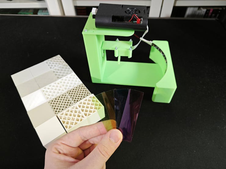
In this regard, I started to inspect various blocking camera filters to pinpoint the wavelength range I required — 100 - 400 nm — by absorbing visible light spectrums. After my research, I decided to utilize two different filter types separately to increase the breadth of UV-applied plastic surface image samples — a glass UV bandpass filter (ZWB ZB2) and color gel filters (with different light transmission levels - low, medium, high).

Since I did not want to constrain my experiments to only one quality control condition by UV-exposure, I decided to employ three different UV light sources providing different wavelengths of ultraviolet radiation — 275 nm, 365 nm, and 395 nm.

✅ DFRobot UVC Ultraviolet Germicidal Lamp Strip (275 nm)

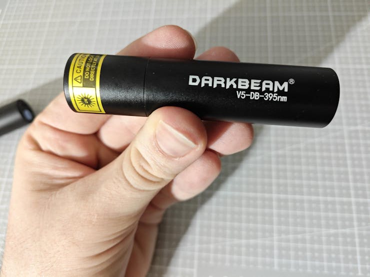
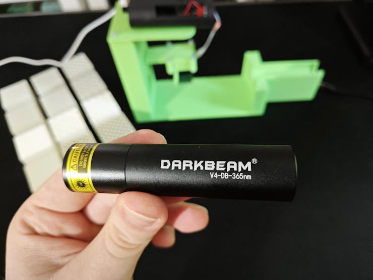
✅ DARKBEAM UV Flashlight (395 nm)

✅ DARKBEAM UV Flashlight (365 nm)

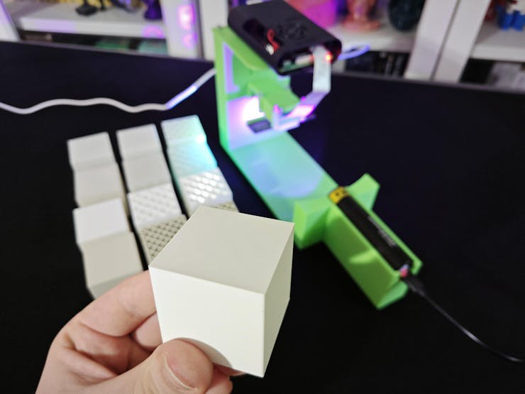
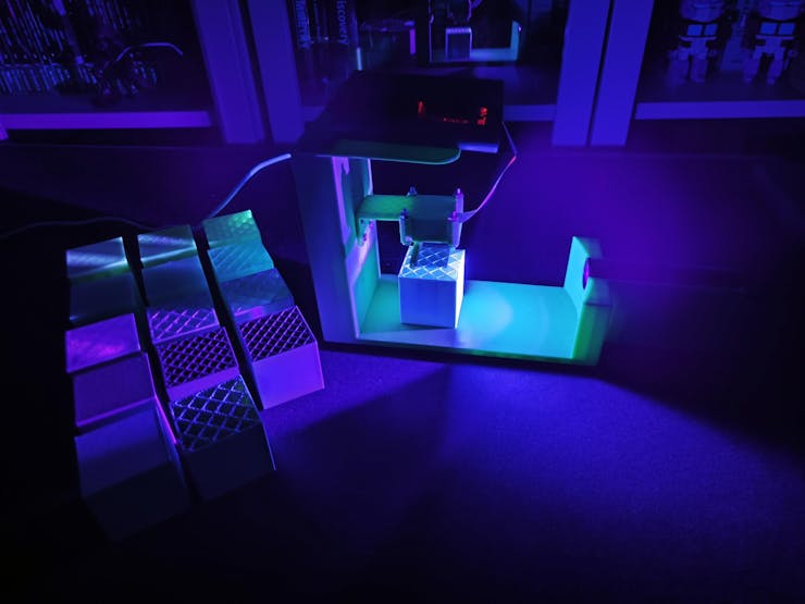
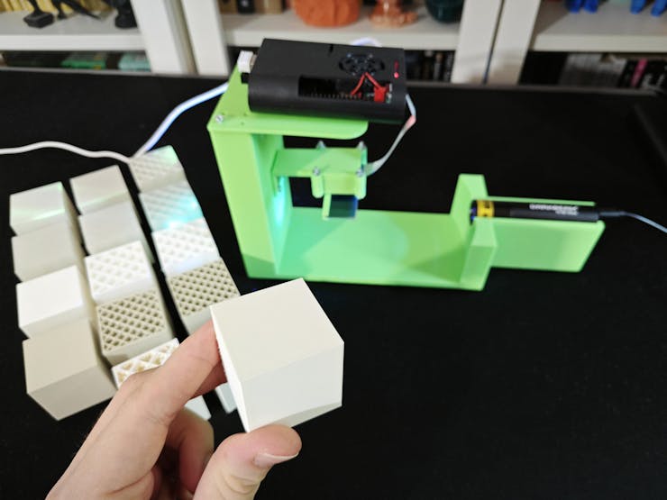
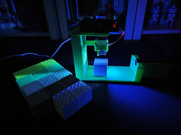
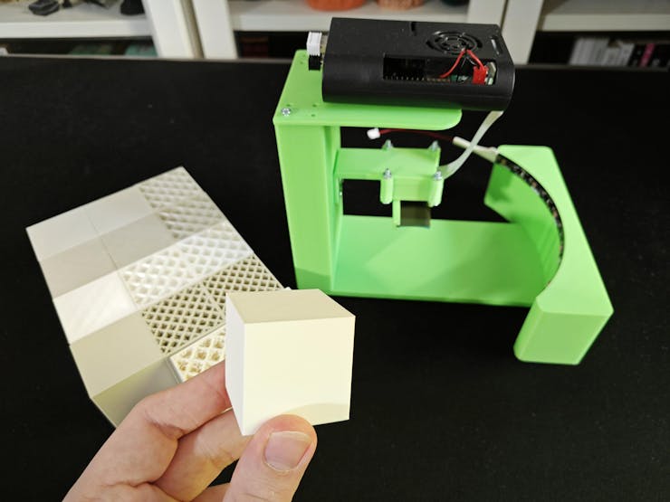
After conceptualizing my initial prototype with the mentioned components, I needed to find an applicable and repeatable method to produce plastic objects with varying stages of surface defects (none, high, and extreme), composed of different plastic materials. After thinking about different production methods, I decided to design a simple cube on Fusion 360 and alter the slicer settings to engender artificial but controlled surface defects (top layer bonding issues). In this regard, I was able to produce plastic objects (3D-printed) with a great deal of variation thanks to commercially available filament types, including UV-sensitive and reflective ones, resulting in an extensive image dataset of UV-applied plastic surfaces.

✅ Matte White

✅ Matte Khaki

✅ Shiny (Silk) White

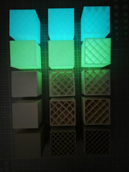
✅ UV-reactive White (Fluorescent Blue)

✅ UV-reactive White (Fluorescent Green)

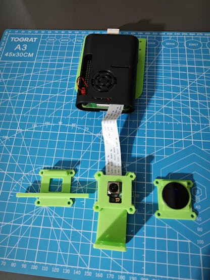
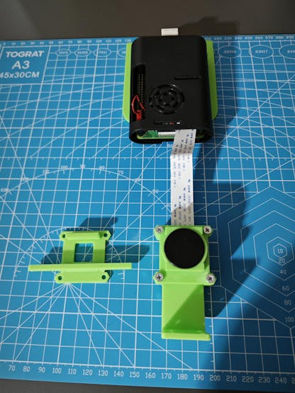
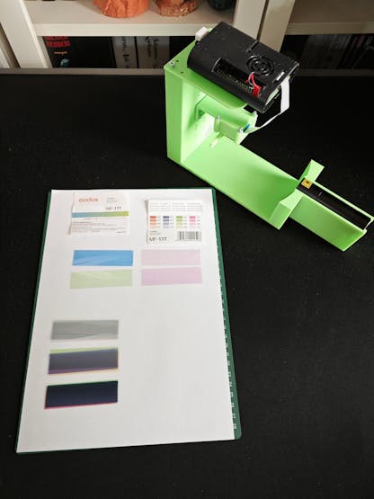
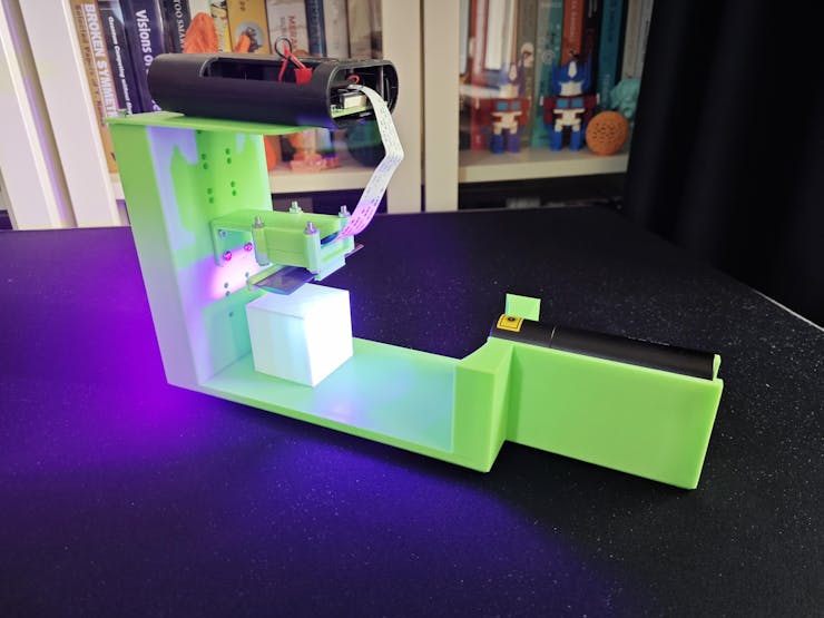
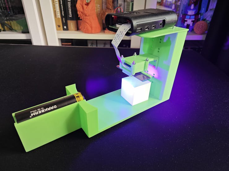
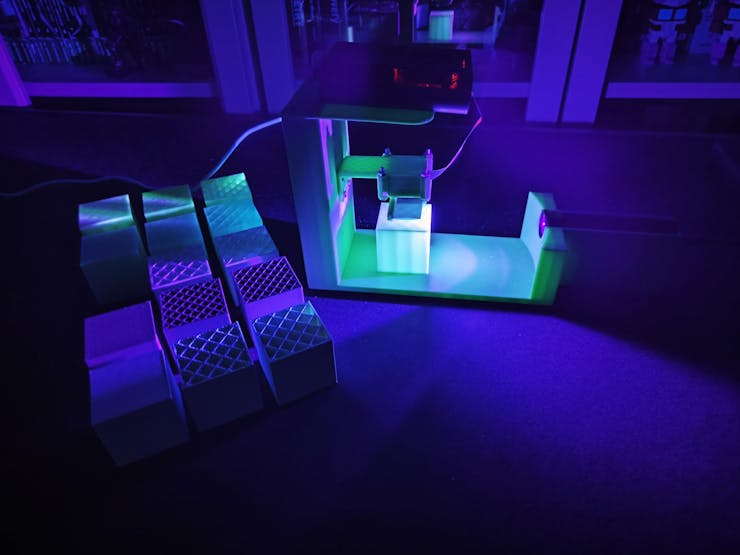
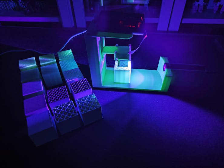
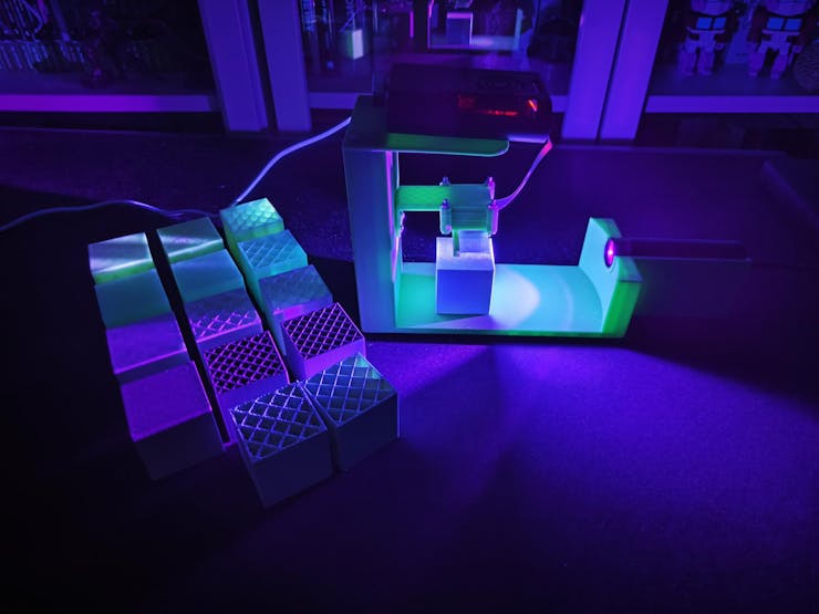
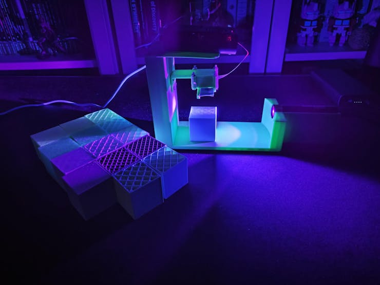
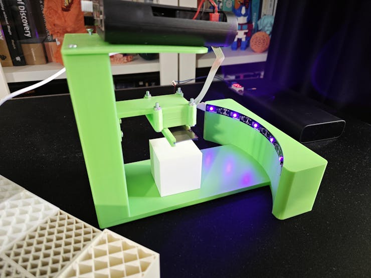
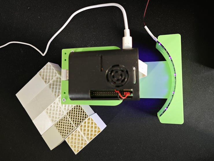
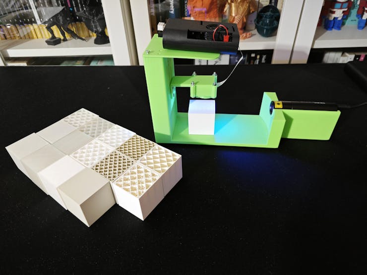
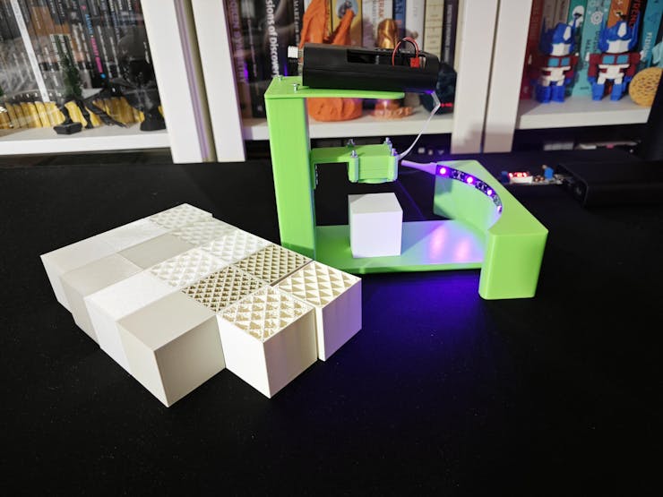
Before proceeding with developing my industrial-grade proof-of-concept device, I needed to ensure that all components, camera filters, UV light sources, and plastic materials (filaments) I chose were compatible and sufficient to generate the UV-applied plastic surface image samples with enough discrepancy (contrast), in accordance with the surface defect stages, to train a visual anomaly detection model. Therefore, I decided to build a simple data collection rig based on Raspberry Pi 4 to construct my dataset and review its validity. As I decided to utilize the Raspberry Pi camera module 3 Wide to cover more of the surface area of the target plastic objects, I designed unique multi-part camera lenses according to its 120° ultra-wide angle of view (AOV) to make the camera module 3 compatible with the glass UV bandpass filter and the color gel filters. Then, I designed two different rig bases (stands) compatible with UV light sources in the flashlight form and the strip form, enabling height adjustment while attaching the camera module case mounts (carrying lenses) to change the distance between the camera (image sensor) focal point and the target plastic object surface.

After building my simple data collection rig, I was able to:

✅ utilize two different types of camera filters — a glass UV bandpass filter (ZWB ZB2) and color gel filters (with different light transmission levels),

✅ adjust the distance between the camera (image sensor) focal point and the plastic object surfaces,

✅ apply three different UV wavelengths — 395 nm, 365 nm, and 275 nm — to the plastic object surfaces,

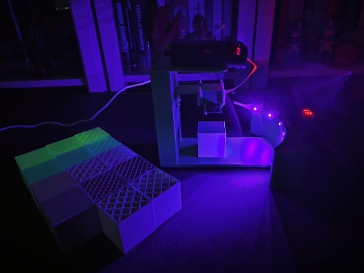
✅ and capture image samples of various plastic materials showcasing three different stages of surface defects — none, high, and extreme — while recording the concurrent experiment parameters.

After collecting UV-applied plastic surface images with all possible combinations of the mentioned experiment parameters, I managed to construct my extensive dataset and achieve a reliable discrepancy between the different surface defect stages to train a visual anomaly detection model. In this regard, I confirmed that the camera module 3 Wide produced sufficient UV-exposed image samples to continue developing my proof-of-concept mechanism.

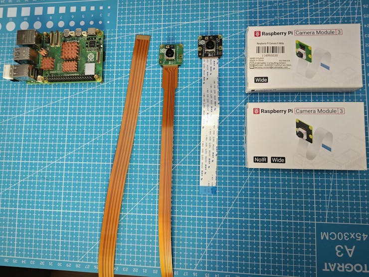
After training and building my FOMO-AD (visual anomaly detection model) on Edge Impulse Studio successfully, I decided not to continue developing my mechanism with the Raspberry Pi 4 and migrated my project to the Raspberry Pi 5 since I wanted to capitalize on the Pi 5’s dual-CSI ports, which allowed me to utilize two different types of camera modules (regular Wide and NoIR Wide) simultaneously. I decided to add the secondary camera module 3 NoIR Wide, which is based on the same IMX708 image sensor but has no IR filter, to review the visual anomaly model behaviour with a regular camera and a night-vision camera simultaneously to develop a feature-rich industrial-grade surface defect detection mechanism.

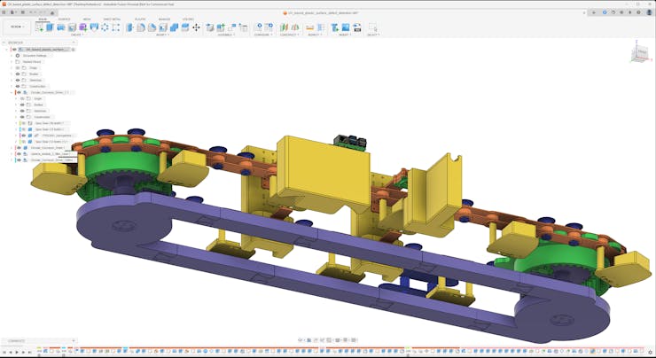
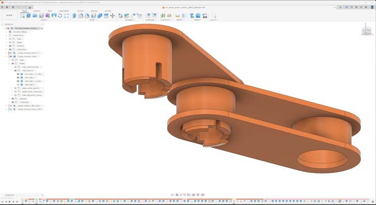
After configuring my dual camera set-up and visual anomaly detection model (FOMO-AD) on Raspberry Pi 5, I started to work on designing a complex circular conveyor mechanism based on my previous data collection rig, letting me place plastic objects under two cameras (regular Wide and NoIR Wide) automatically and run inferences with the images produced by them simultaneously.

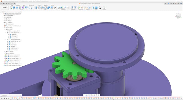
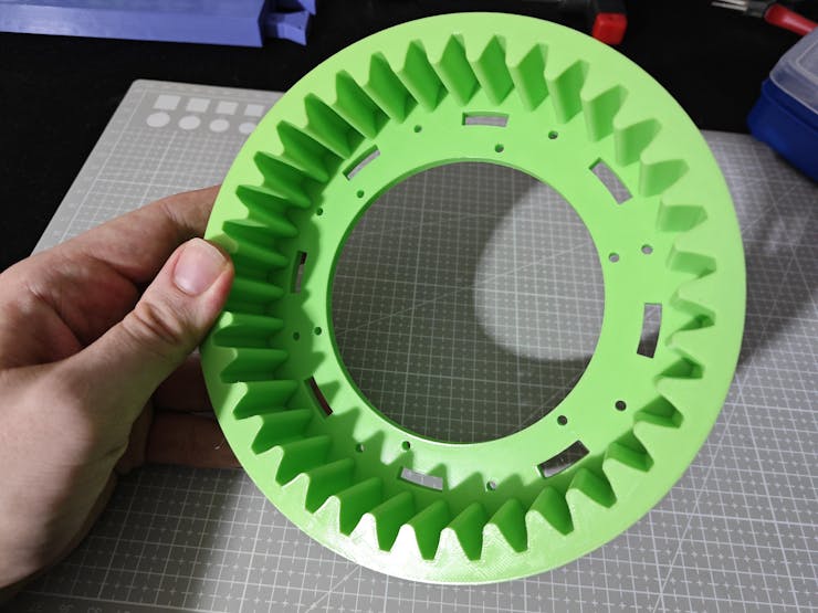
Since I wanted to develop a sprocket-chain circular conveyor mechanism rather than a belt-driven one, I needed to design a lot of custom mechanical components to achieve my objectives and conduct fruitful experiments. Since I wanted to apply a different approach rather than limit switches to align plastic objects under the focal points of the cameras, I decided to utilize neodymium magnets and two magnetic Hall-effect sensor modules. While building these complex parts, I encountered various issues and needed to go through different iterations to complete my conveyor mechanism until I was able to demonstrate the features I planned. I documented my design mistakes and adjustments below to explain my development process thoroughly for this research study :)

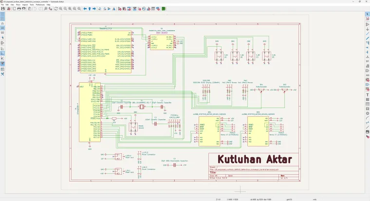
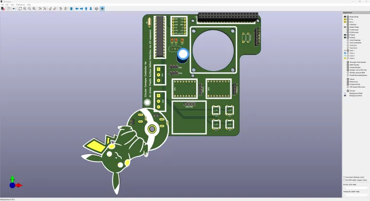
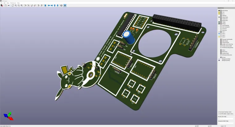
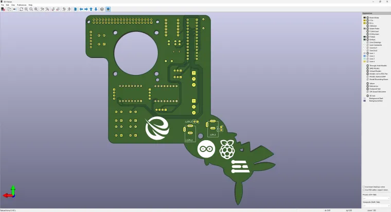
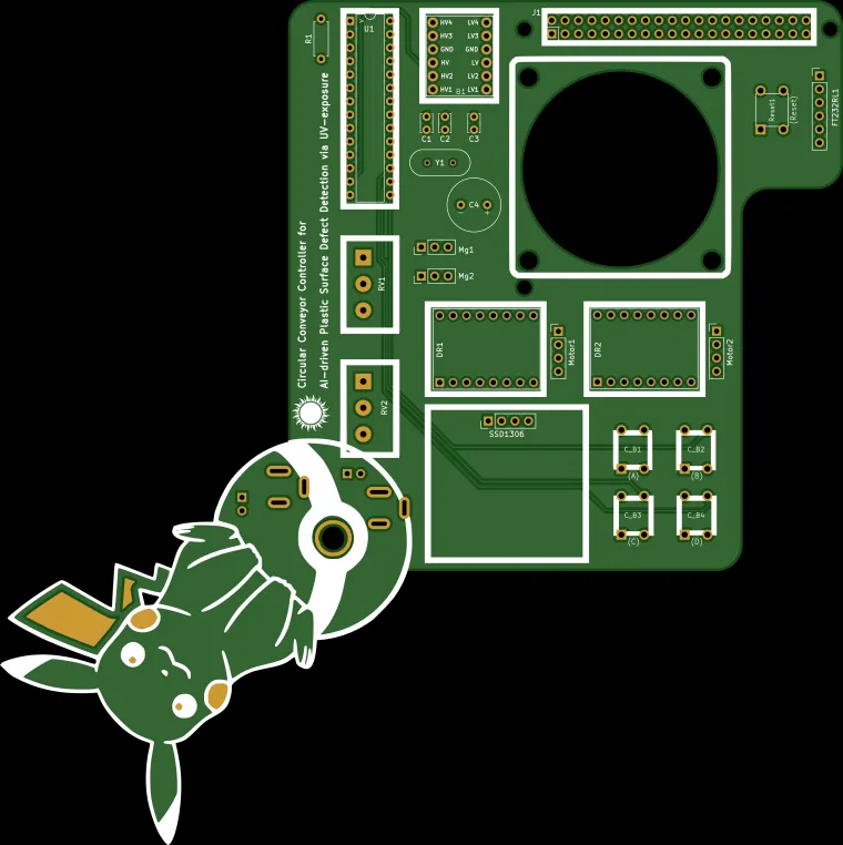
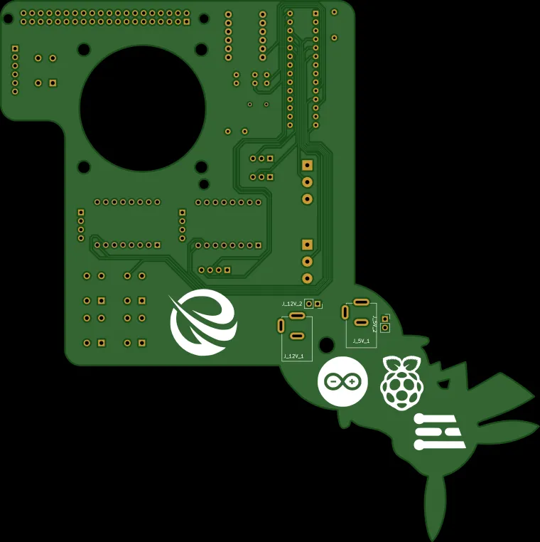
As I was starting to design the mechanical components, I decided to develop a unique controller board (PCB) as the primary interface of the sprocket-chain circular conveyor. To reduce the footprint of the controller board, I decided to utilize an ATmega328P and design the controller board (4-layer PCB) as a custom Raspberry Pi 5 shield (hat).

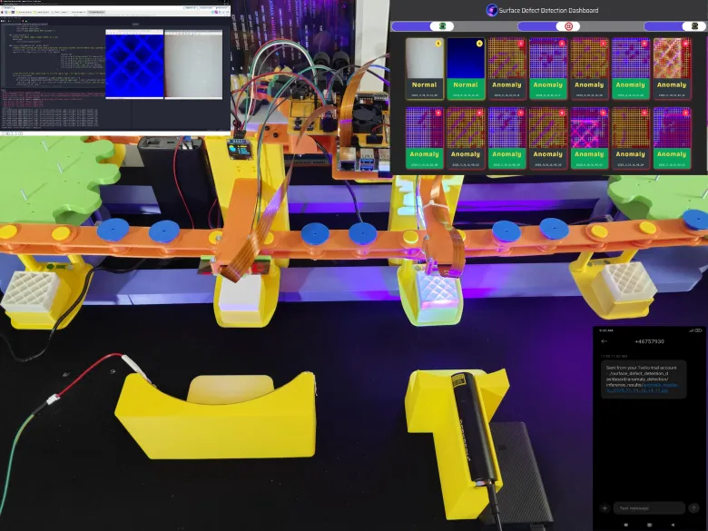
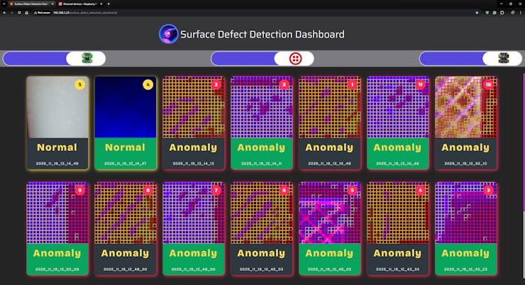
Finally, since I wanted to simulate the experience of operating an industrial-grade automation system, I developed an authentic web dashboard for the circular conveyor, which lets the user:

✅ review real-time inference results with timestamps,

✅ sort the inference results by camera type (regular or NoIR),

✅ and enable the Twilio integration to get the latest surface anomaly detection notifications as SMS.

By referring to the following tutorial, you can inspect the in-depth feature, design, and code explanations with the challenges I faced during the overall development process.

 

 

 

Development process, different prototype versions, design failures, and final results

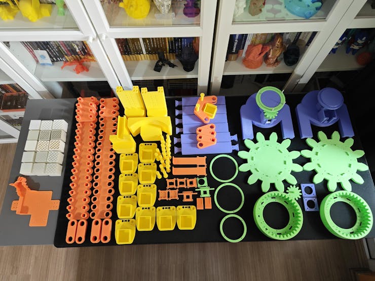
As I was developing this research project, I encountered lots of problems due to complex mechanical component designs, especially related to the sprocket-chain mechanism, leading me to go through five different iterations. I documented the overall development process for the final mechanism in the following written tutorial thoroughly and showcased the features of the final version in the project demonstration videos.

 

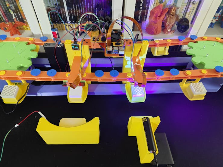
Every feature of the final version of this proof-of-concept automation mechanism worked as planned and anticipated after my adjustments, except that the stepper motors (Nema 17) around which I designed the primary internal gears could not handle the extra torque applied to my custom-designed ball bearings (with 5 mm steel beads) after I recalibrated the chain tension with additional tension pins. I explained the reasons for the tension recalibration thoroughly in the following steps. In this regard, I needed to record some features related to sprocket movements (affixed to outer gears pivoted on the ball bearings) by removing or loosening the chain for the demonstration videos.

Data Collection Rig - Step 1: Defining the parameters for this research study, planning experiments, and outlining the research roadmap

As I briefly talked about my thought process for deciding the experiment parameters and sourcing components in the introduction, I will thoroughly cover the progress of building the UV-applied plastic surface image sample (data) collection rig in this section.

The simple data collection rig is the first version of this research project, which helped me to ensure that all components, camera filters, UV light sources, and plastic materials (filaments) I chose were compatible and sufficient to produce an extensive UV-applied plastic surface image dataset with enough discrepancy (contrast) to train a visual anomaly detection model.

As mentioned, after meticulously inspecting the documentation of various commercially available camera sensors, I decided to employ the Raspberry Pi camera module 3 Wide (120°) to capture images of plastic surfaces, showcasing different surface defect stages, under varying UV wavelengths. I studied the spectral sensitivity of the CMOS 12-megapixel Sony IMX708 image sensor and other available Raspberry Pi camera modules on the official Raspberry Pi camera documentation.

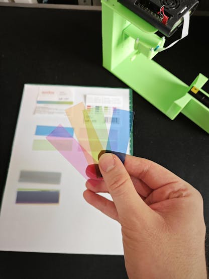
Since I decided to benefit from external camera filters to capture UV-oriented image samples with enough discrepancy (contrast) in accordance with the inherent surface defects, instead of heavily modifying the Bayer layer and the integrated camera filters, I sourced nearly full-spectrum color gel filters with different light transmission levels for blocking visible light. By stacking up these color gel filters, I managed to capture accurate UV-induced plastic surface images in the dark.

• Godox color gel filters with low light transmission
• Godox color gel filters with medium light transmission
• Godox color gel filters with high light transmission

Of course, only utilizing visible light-blocking color gel filters was not enough, considering the extent of this research study. In this regard, I also sourced a precise glass UV bandpass filter absorbing the visible light spectrum. Although I inspected the glass bandpass filter specifications from a different brand's documentation, I was only able to purchase one from AliExpress.

• UV bandpass filter (25 mm glass ZWB ZB2)

As I did not want to constrain this research project to showcase only one UV light source type while experimenting with quality control conditions by the direct application of UV (ultraviolet radiation) to plastic object surfaces, I decided to purchase three different UV light sources providing different UV wavelength ranges.

• DFRobot UVC Ultraviolet Germicidal Lamp Strip (275 nm)
• DARKBEAM UV Flashlight (395 nm)
• DARKBEAM UV Flashlight (365 nm)

Since I decided to manufacture plastic objects myself to control experiment parameters to develop a valid research project, I needed to find an applicable and repeatable method to produce plastic objects with varying stages of surface defects (none, high, and extreme) and source different plastic materials to produce a wide selection of plastic objects. After mulling over different production methods, I decided to produce my plastic objects with 3D printing and modify slicer settings to inflict artificial but controllable surface defects. Thanks to commercially available filament types, including UV-sensitive and reflective ones, I was able to source a great variety of materials to construct an extensive image dataset of UV-applied plastic surfaces.

• ePLA-Matte Milky White
• ePLA-Matte Light Khaki
• eSilk-PLA White (Shiny)
• PLA+ Luminous Green (UV-reactive - Fluorescent)
• PLA+ Luminous Blue (UV-reactive - Fluorescent)

#️⃣ First, I designed a simple cube on Autodesk Fusion 360 with dimensions of 40.00 mm x 40.00 mm x 40.00 mm.

#️⃣ I exported the cube as an STL file and uploaded the exported STL file to Bambu Studio.

#️⃣ Then, I modified the slicer (Bambu Studio) settings to implement artificial surface defects, in other words, inflicted top-layer bonding issues.

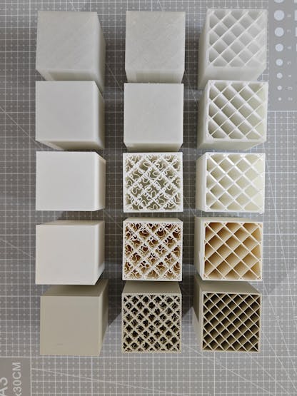
#️⃣ Since I wanted to showcase three different surface defect stages — none, high, and extreme — I copied the cube three times on the slicer.

#️⃣ For all three cubes, I selected the sparse infill density as 10% to outline the inflicted surface defects.

#️⃣ I utilized the standard slicer settings for the first cube, depicting the none surface defect stage.

#️⃣ For the second cube, I reduced the top shell layer number to 0 and selected the top surface pattern as the monotonic line, representing the extreme surface defect stage.

#️⃣ For the third cube, I lowered the top shell layer number to 1 and selected the top surface pattern as the Hilbert curve, representing the high surface defect stage.

#️⃣ However, as shown in the print preview, only reducing the top shell layer number would not lead to a protruding high defect stage, as I had hoped. Thus, I also reduced the top shell thickness to 0 to get the results I anticipated.

#️⃣ Since I decided to add the matte light khaki filament latest, I sliced three khaki cubes with 15% sparse infill density to expand my plastic object sample size.

After meticulously printing the three cubes showcasing different surface defect stages with each filament, I produced all plastic objects (15 in total) required to construct an extensive dataset to train a visual anomaly detection model and develop my industrial-grade proof-of-concept surface defect detection mechanism.

 

 

 

Data Collection Rig - Step 2: Designing unique camera lenses compatible with UV bandpass filter and color gel filters

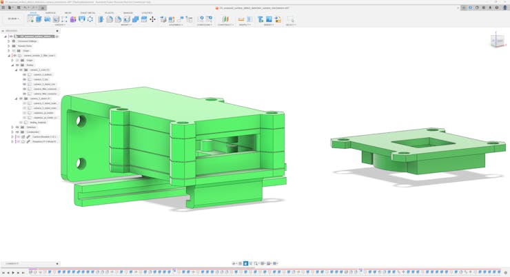
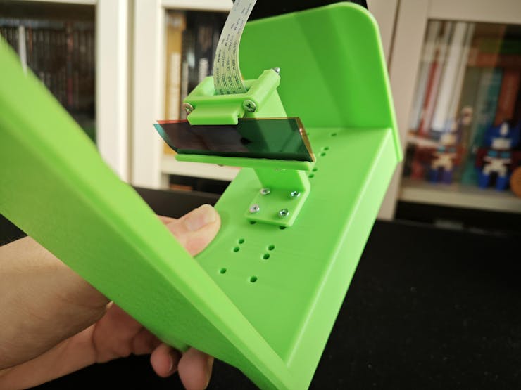
Since I wanted to utilize external filters not compatible with the camera module 3 Wide, I needed to design unique camera lenses housing the color gel filters and the glass UV bandpass filter. In the case of gel filters, I had to design the camera lens to make color gel filters hot swappable while experimenting with different light transmission levels - low, medium, and high. Conversely, in the case of the glass bandpass, I had to design the camera lens as rigid as possible to avoid any light reaching the image sensor without passing through the bandpass filter. On top of all of these lens requirements, I also had to make sure that the color gel and the UV bandpass filter lenses were easily changable during my experiments.

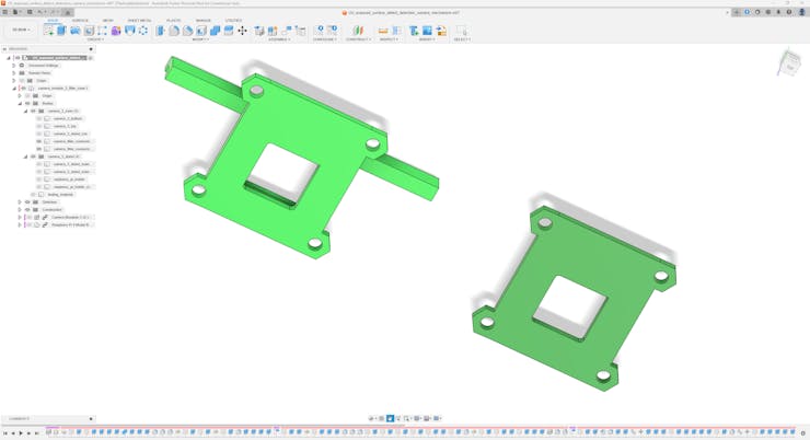
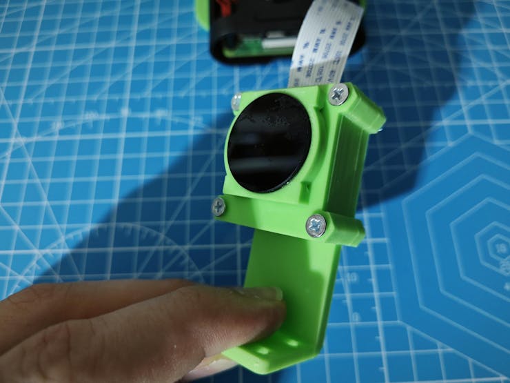
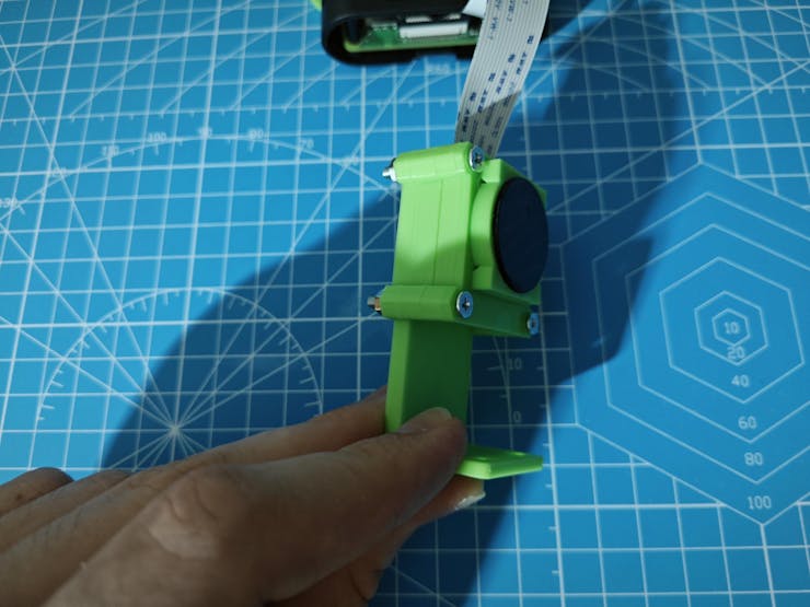
After sketching different lens arrangements, I decided to design a unique multi-part case for the camera module 3, which gave me the freedom to design lenses with minimal alterations to the base of the camera case and mount.

As I was working on these components, I leveraged some open-source CAD files to obtain accurate measurements:

✒️ Raspberry Pi Camera Module v3 (Step) | Inspect

✒️ Raspberry Pi 4 Model B (Step) | Inspect

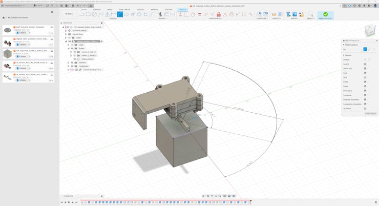
#️⃣ First, I designed the camera module case, mount, and lens for the color gel filters on Fusion 360.

#️⃣ Since the camera module 3 Wide has a 120° ultra-wide angle of view (AOV), I aligned the focal point of the image sensor and the horizontal borders of the lens accordingly.

#️⃣ After completing the focal point alignment, I designed the glass UV bandpass filter lens by altering the color gel filter lens to protect the 120-degree horizontal border placement.

#️⃣ Since the camera module case is composed of stackable parts, it can be utilized without adding the filter lenses as a stand-alone case.

After completing the camera module case, mount, and lens designs, I started to work on the placement of the camera module in relation to the target plastic object surface and the applied UV light source. To capture a precise UV-exposed image highlighting as many plastic surface defects as possible, I needed to make sure that the camera module's image sensor (IMX708) would catch the reflected ultraviolet radiation as optimally as possible during my experiments.

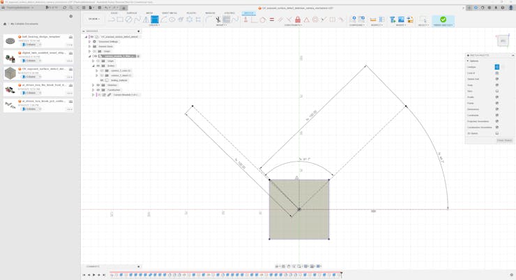
In this regard, I needed to align the focal point of the camera sensor and the focal point of the applied UV light source on perpendicular axes, intersecting at the center of the UV-applied plastic surface. Since I selected UV light sources in the flashlight and strip formats, the most efficient way to place my light sources was to calculate the arc angle required to create a concave (converging) shape to focus the ultraviolet radiation emitted by the UVC strip (275 nm) directly to the center of the target plastic surface. By knowing the center (focal point) of the calculated arc, I could easily place the remaining UV flashlights directly pointed at the center of the target plastic object.

#️⃣ As I decided to place UV light sources ten centimeters (100 mm) away from plastic objects and knew the length of the UVC strip, I was able to calculate the required arc angle effortlessly via this formula:

S = r * θ

S ➡ Arc length [length of the UVC strip]

r ➡ Radius [distance between the center of the plastic object surface and the arc center (focal point)]

θ➡ Central angle in radians [angle/rad]

Arc_angle = (Arc_length * rad) / Radius

 

 

 

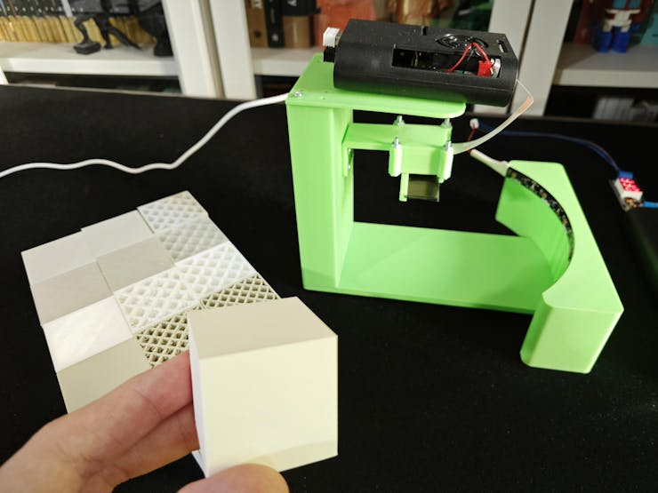
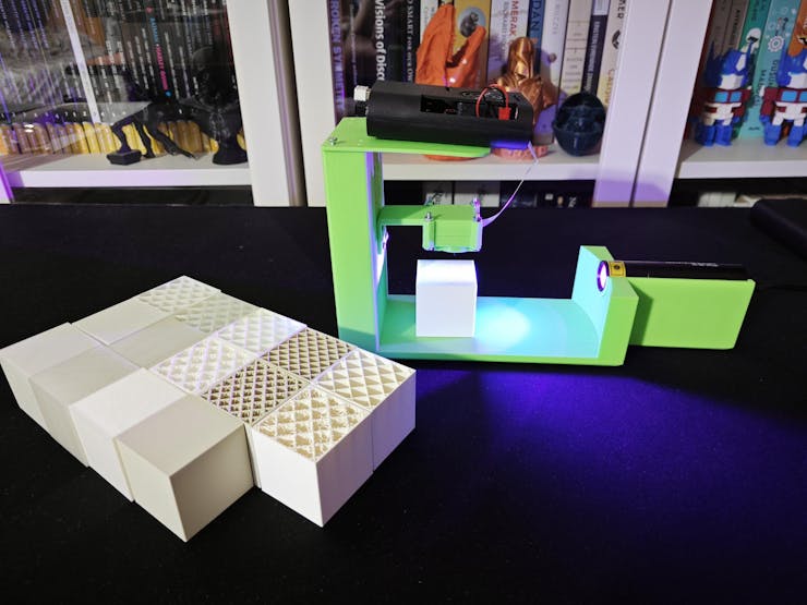
Data Collection Rig - Step 3: Designing the rig bases (stands) compatible with UV flashlights and strips

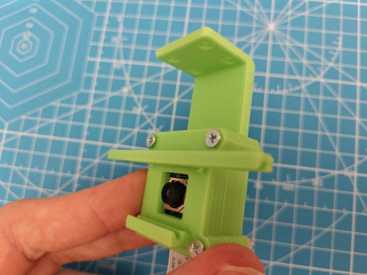
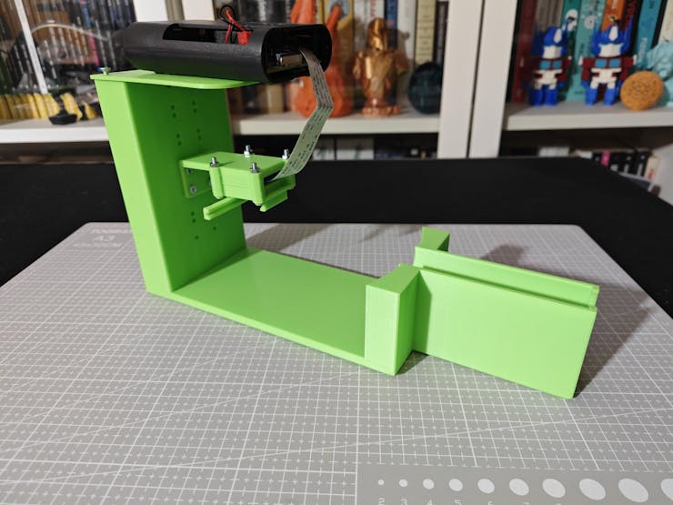
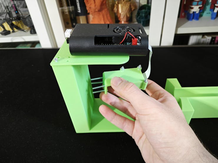
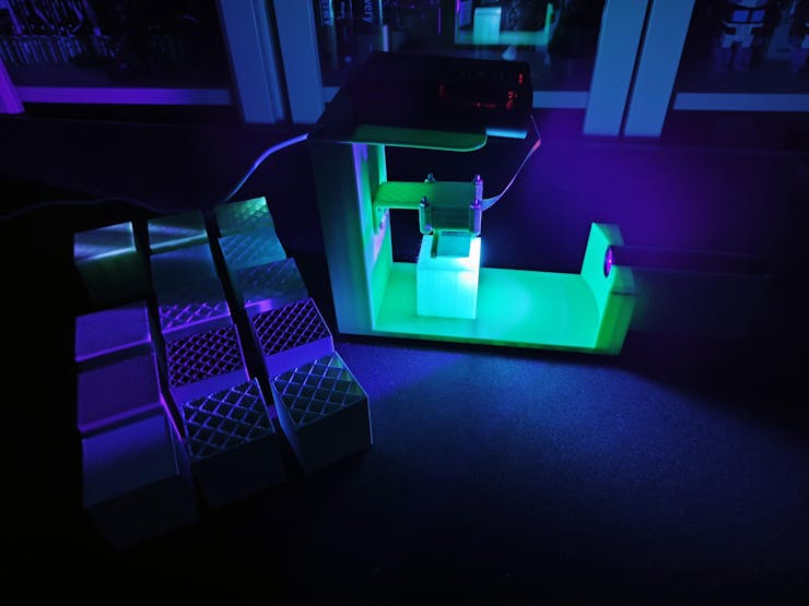
After calculating the arc angle, I continued to design the rig base compatible with the UVC strip, providing the concave (converging) shape to focus the emitted ultraviolet radiation directly onto the target plastic object surface. Based on the camera module mount, the rear part of the camera module case, I added a rack to the rig base to enable different levels (height adjustment) while attaching the camera module case (mount) to the rig base. In this regard, the rig base lets the user change the distance between the camera (image sensor) focal point and the target plastic object surface effortlessly.

I also added a simple holder to place the Raspberry Pi 4 on the top of the rig base easily while positioning the camera module case, providing hex-shaped snug-fit peg joints for easy installation.

As mentioned earlier, by knowing the center (focal point) of the calculated arc, I was able to modify the concave shape of the rig base for the UVC strip to design a subsequent rig base compatible with the remaining UV light sources in the flashlight format.

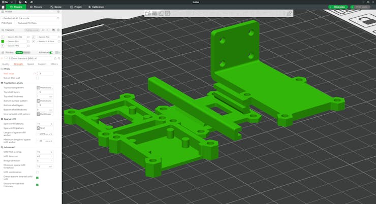
#️⃣ After completing the overall rig design, I exported all parts as STL files and uploaded them to Bambu Studio.

#️⃣ To boost the rigidity of the camera module case parts to produce a sturdy frame while experimenting with the external camera filters, I increased the wall loop (perimeter) number to 3.

#️⃣ To precisely place tree supports, I utilized support blockers while slicing the flashlight rig base.

 

 

 

Data Collection Rig - Step 4: Assembling the data collection rig and the custom camera filter lenses

After printing all of the data collection rig parts with my Bambu Lab A1 Combo, which helped me a lot while printing the plastic objects with different filaments, thanks to the integrated AMS lite.

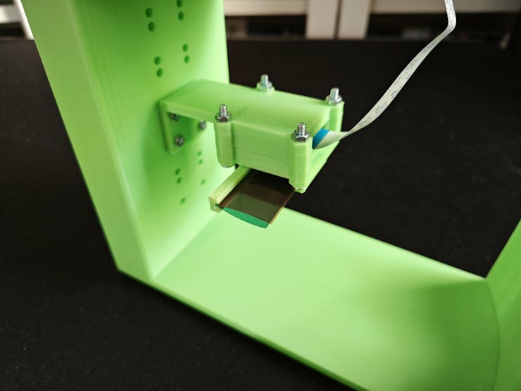
#️⃣ First, I started to assemble the multi-part camera module case. Since I designed all case parts stackable to swap external camera filters without changing the case frame, I was able to assemble the whole case with four M3 screw-nut pairs.

#️⃣ Since I specifically designed the external color gel filter camera lens to make gel filters hot swappable while experimenting with different light transmission levels — low, medium, and high — I was able to affix the gel camera lens directly to the case frame.

#️⃣ After completing the assembly of the camera module case with the external gel filter lens, I connected the camera module 3 to the Raspberry Pi 4 via an FFC cable (150 mm) to test the fidelity of the captured images.

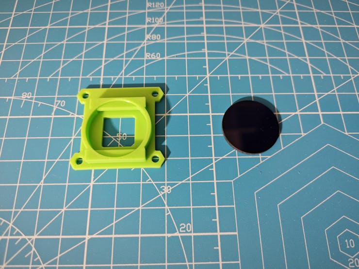
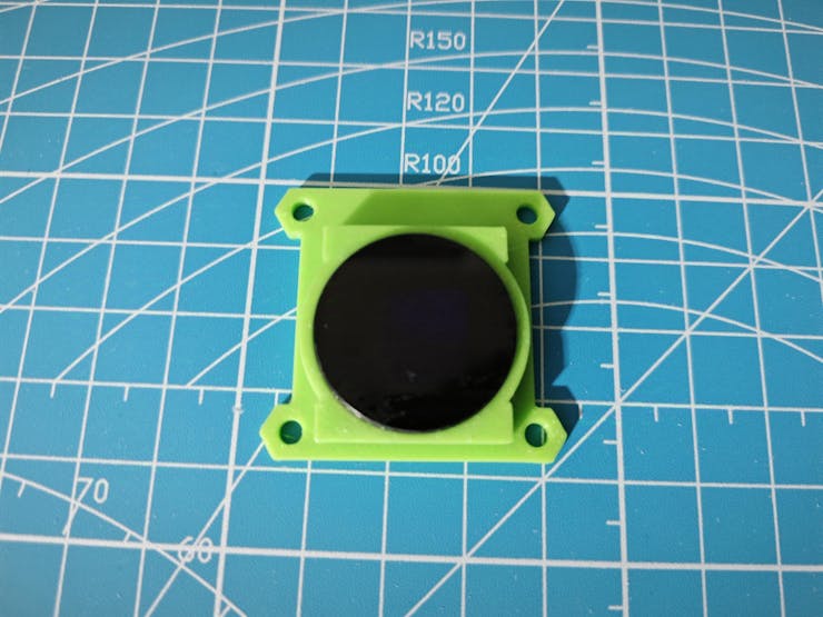
#️⃣ On the other hand, as discussed, I designed the external UV bandpass filter camera lens as rigid as possible to avoid any light reaching the image sensor without passing through the glass UV bandpass filter. Therefore, I diligently applied instant glue (super glue) to permanently affix the glass bandpass filter to its unique camera lens.

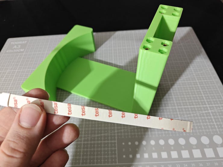
#️⃣ After installing M3 brass threaded inserts with my TS100 soldering iron to strengthen the connection between the rig bases and the Raspberry Pi 4 holder, I continued to attach the UV light sources to their respective rig bases.

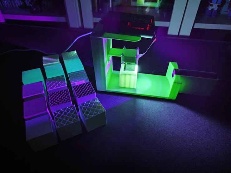
#️⃣ As the 275 nm UVC strip (FPC circuit board) came with an adhesive tape side, I was able to fasten the UVC strip to the dedicated concave shape of the rig base effortlessly.

#️⃣ As I specifically designed the subsequent rig base considering the measurements of my UV light sources in the flashlight format (395 nm and 365 nm), the installation of UV flashlights was as easy as sliding them into their dedicated slot.

#️⃣ After installing the UV light sources into their respective rig bases successfully, to initiate my preliminary experiments, I attached the camera module case to the rack of the UV flashlight-compatible rig base by utilizing four M3 screw-nut pairs.

#️⃣ Then, I attached the Raspberry Pi 4 holder to the top of the rig base via M3 screws through the peg joints and placed the Raspberry Pi 4 onto its holder.

 

 

 

 

Data Collection Rig - Step 5: Setting up and programming Raspberry Pi 4 to capture images with the camera module 3 while logging the applied experiment parameters

As you might have noticed, I have always explained setting up the Raspberry Pi OS in my previous tutorials. Nonetheless, the latest version of the Raspberry Pi Imager is very straightforward to the point of letting the user configure the SSH authentication method and the Wi-Fi credentials. You can inspect the official Raspberry Pi Imager documentation here.

#️⃣ After setting up Raspberry Pi OS successfully, I installed the required Python modules (libraries) to continue developing.

sudo apt-get update

sudo apt-get install python3-opencv

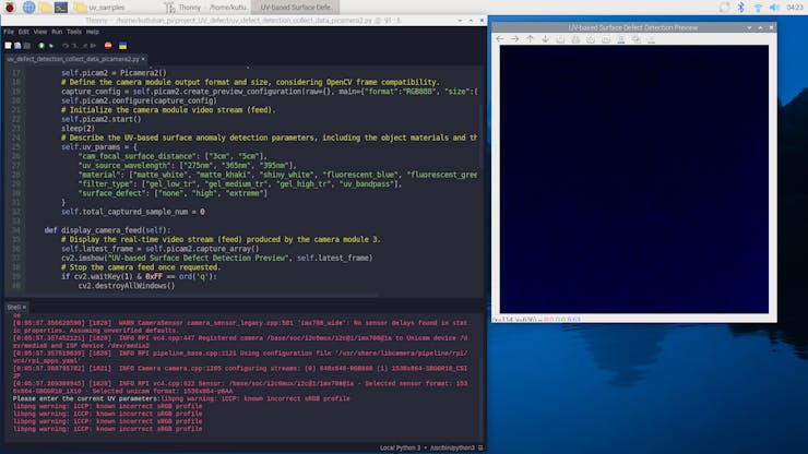
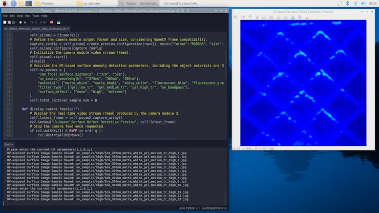
#️⃣ After updating the system and installing the required libraries, I started to work on the Python script to capture UV-applied plastic surface image samples and allow the user to record the concurrent experiment parameters to the image file names by entering user inputs.

📁 uv_defect_detection_collect_data_w_rasp_4_camera_mod_wide.py

⭐ Include the required system and third-party libraries.

⭐ Uncomment to modify the libcamera log level to bypass the libcamera warnings if you want clean shell messages while entering user inputs.

import cv2
from picamera2 import Picamera2, Preview
from time import sleep
from threading import Thread

# Uncomment to disable libcamera warnings while collecting data.
#import os
#os.environ["LIBCAMERA_LOG_LEVELS"] = "4"

#️⃣ To bundle all the functions to write a more concise script, I used a Python class.

⭐ In the __init__ function:

⭐ Define a picamera2 object for the Raspberry Pi camera module 3 Wide.

⭐ Define the output format and size (resolution) of the captured images to obtain an OpenCV-compatible buffer — RGB888. Then, configure the picamera2 object accordingly.

⭐ Initialize the video stream (feed) produced by the camera module 3.

⭐ Describe all possible experiment parameters in a Python dictionary for easy access.

class uv_defect_detection():
    def __init__(self):
        # Define the Raspberry Pi camera module 3 object.
        self.picam2 = Picamera2()
        # Define the camera module output format and size, considering OpenCV frame compatibility.
        capture_config = self.picam2.create_preview_configuration(raw={}, main={"format":"RGB888", "size":(640,640)})
        self.picam2.configure(capture_config)
        # Initialize the camera module video stream (feed).
        self.picam2.start()
        sleep(2)
        # Describe the UV-based surface anomaly detection parameters, including the object materials and the applied camera filter types.
        self.uv_params = {
            "cam_focal_surface_distance": ["3cm", "5cm"],
            "uv_source_wavelength": ["275nm", "365nm", "395nm"],
            "material": ["matte_white", "matte_khaki", "shiny_white", "fluorescent_blue", "fluorescent_green"],
            "filter_type": ["gel_low_tr", "gel_medium_tr", "gel_high_tr", "uv_bandpass"],
            "surface_defect": ["none", "high", "extreme"]           
        }
        self.total_captured_sample_num = 0
		
		...

⭐ In the display_camera_feed function:

⭐ Obtain the latest frame generated by the camera module 3.

⭐ Then, show the obtained frame on the screen via the built-in OpenCV tools.

⭐ Stop the camera feed and terminate the OpenCV windows once requested.

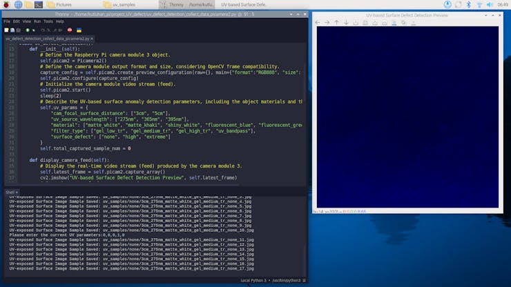
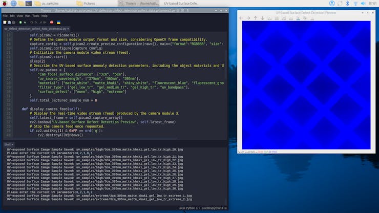
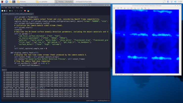
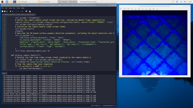
def display_camera_feed(self):
        # Display the real-time video stream (feed) produced by the camera module 3.
        self.latest_frame = self.picam2.capture_array()
        cv2.imshow("UV-based Surface Defect Detection Preview", self.latest_frame)
        # Stop the camera feed once requested.
        if cv2.waitKey(1) & 0xFF == ord('q'):
            cv2.destroyAllWindows()
            self.picam2.stop()
            self.picam2.close()
            print("\nCamera Feed Stopped!")

⭐ In the camera_feed function, initiate the loop to show the latest frames consecutively to observe the real-time video stream (feed).

def camera_feed(self):
        # Start the camera video stream (feed) loop.
        while True:
            self.display_camera_feed()

⭐ In the save_uv_img_samples function:

⭐ Define the file name and path of the current image sample by applying the passed experiment parameters.

⭐ Up to the passed batch number, save the latest successive frames with the given file name and path, differentiated by the sample number.

⭐ Wait half a second before obtaining the next available frame.

def save_uv_img_samples(self, params, batch):
        # Based on the provided UV parameters, create the image sample name.
        img_file = "uv_samples/{}/{}_{}_{}_{}_{}".format(self.uv_params["surface_defect"][int(params[4])],
                                                         self.uv_params["cam_focal_surface_distance"][int(params[0])],
                                                         self.uv_params["uv_source_wavelength"][int(params[1])],
                                                         self.uv_params["material"][int(params[2])],
                                                         self.uv_params["filter_type"][int(params[3])],
                                                         self.uv_params["surface_defect"][int(params[4])]
                                                         )
        # Save the latest frames captured by the camera module consecutively according to the passed batch number.
        for i in range(batch):
            self.total_captured_sample_num += 1
            if (self.total_captured_sample_num > 30): self.total_captured_sample_num = 1
            _img_file = img_file + "_{}.jpg".format(self.total_captured_sample_num)
            cv2.imwrite(_img_file, self.latest_frame)
            # Wait before getting the next available frame.
            sleep(0.5)
            print("UV-exposed Surface Image Sample Saved: " + _img_file)

⭐ In the obtain_and_decode_input function:

⭐ Initiate the loop to obtain user inputs continuously.

⭐ Once the user input is fetched, decode the retrieved string to obtain the given experiment parameters as an array. Then, check the number of the extracted experiment parameters.

⭐ If matched, capture image samples up to the given batch number (10) and record the given experiment parameters to the sample file names.

def obtain_and_decode_input(self):
        # Initiate the user input prompt to obtain the current UV parameters to capture image samples.
        while True:
            passed_params = input("Please enter the current UV parameters:")
            # Decode the passed string to extract the provided UV parameters.
            decoded_params = passed_params.split(",")
            # Check the number of the given parameters.
            if (len(decoded_params) == 5):
                # If matched, capture image samples according to the passed batch number.
                self.save_uv_img_samples(decoded_params, 10)
            else:
                print("Wrong parameters!")

#️⃣ As the built-in Python input function needs to check for new user input without interruptions, it cannot run with the real-time video stream generated by OpenCV in the same operation (runtime), which processes the latest frames produced by the camera module 3 continuously. Therefore, I utilized the built-in Python threading module to run multiple operations concurrently and synchronize them.

⭐ Define the uv_defect_detection class object.

⭐ Declare and initialize a Python thread for running the real-time video stream (feed).

⭐ Outside of the video stream operation (thread), check new user inputs continuously to obtain the provided experiment parameters.

uv_defect_detection_obj = uv_defect_detection()

# Declare and initialize Python thread for the camera module video stream (feed).
Thread(target=uv_defect_detection_obj.camera_feed).start()

# Obtain the provided UV parameters as user input continuously.
uv_defect_detection_obj.obtain_and_decode_input()

 

 

 

Data Collection Rig - Step 6: Constructing an extensive image dataset of surfaces of various plastic materials with different defect states under 395 nm, 365 nm, and 275 nm UV wavelengths

After concluding programming the Raspberry Pi 4, I proceeded to capture UV-applied plastic surface image samples showcasing all of the combinations of the experiment parameters to construct my extensive dataset.

I would like to reiterate all experiment parameters to elucidate the extent of the completed image dataset.

#️⃣ I utilized three different UV light (radiation) sources, providing varying wavelength ranges.

• 275 nm
• 365 nm
• 395 nm

#️⃣ I designed three cubes showcasing different surface defect stages.

• none
• high
• extreme

#️⃣ I printed these three cubes with five different plastic materials (filaments) to increase my sample size.

• Matte White
• Matte Khaki
• Shiny (Silk) White
• UV-reactive White (Fluorescent Blue)
• UV-reactive White (Fluorescent Green)

#️⃣ I applied two different types of external camera filters, making it four different filter options due to the gel filters' light transmission levels.

• UV bandpass filter (glass)
• Gel filters with low light transmission
• Gel filters with medium light transmission
• Gel filters with high light transmission

#️⃣ I stacked up four different primary colors provided by my gel filter set to pass the required blue-oriented wavelength range and block the remaining visible light spectrums.

#️⃣ Since my color gel filter set included three gel filters for each primary color with varying light transmission levels, I decided to use low, medium, and high color gel filter groups, sets of four primary colors, during my experiments.

#️⃣ Since I specifically designed the rig base racks to be able to attach the camera module case mounts (carrying external lenses) at different height levels, I was able to adjust the distance between the camera (image sensor) focal point and the target plastic object surface. In this regard, I collected image samples at two different height levels to acquire samples with different zoom percentages.

• 3 cm
• 5 cm

#️⃣ Considering all of the mentioned experiment parameters, I painstakingly collected UV-applied plastic surface image samples with every possible combination and constructed my extensive dataset successfully.

• none / 3 cm / 395 nm / Gel (low transmission)
• high / 3 cm / 395 nm / Gel (low transmission)
• extreme / 3 cm / 395 nm / Gel (low transmission)
• none / 3 cm / 395 nm / Gel (medium transmission)
• high / 3 cm / 395 nm / Gel (medium transmission)
• extreme / 3 cm / 395 nm / Gel (medium transmission)
• none / 3 cm / 395 nm / Gel (high transmission)
• high / 3 cm / 395 nm / Gel (high transmission)
• extreme / 3 cm / 395 nm / Gel (high transmission)
• none / 3 cm / 395 nm / UV bandpass
• high / 3 cm / 395 nm / UV bandpass
• extreme / 3 cm / 395 nm / UV bandpass
• none / 3 cm / 365 nm / Gel (low transmission)
• high / 3 cm / 365 nm / Gel (low transmission)
• extreme / 3 cm / 365 nm / Gel (low transmission)
• none / 3 cm / 365 nm / Gel (medium transmission)
• high / 3 cm / 365 nm / Gel (medium transmission)
• extreme / 3 cm / 365 nm / Gel (medium transmission)
• none / 3 cm / 365 nm / Gel (high transmission)
• high / 3 cm / 365 nm / Gel (high transmission)
• extreme / 3 cm / 365 nm / Gel (high transmission)
• none / 3 cm / 365 nm / UV bandpass
• high / 3 cm / 365 nm / UV bandpass
• extreme / 3 cm / 365 nm / UV bandpass
• none / 3 cm / 275 nm / Gel (low transmission)
• high / 3 cm / 275 nm / Gel (low transmission)
• extreme / 3 cm / 275 nm / Gel (low transmission)
• none / 3 cm / 275 nm / Gel (medium transmission)
• high / 3 cm / 275 nm / Gel (medium transmission)
• extreme / 3 cm / 275 nm / Gel (medium transmission)
• none / 3 cm / 275 nm / Gel (high transmission)
• high / 3 cm / 275 nm / Gel (high transmission)
• extreme / 3 cm / 275 nm / Gel (high transmission)
• none / 3 cm / 275 nm / UV bandpass
• high / 3 cm / 275 nm / UV bandpass
• extreme / 3 cm / 275 nm / UV bandpass
• none / 5 cm / 395 nm / Gel (low transmission)
• high / 5 cm / 395 nm / Gel (low transmission)
• extreme / 5 cm / 395 nm / Gel (low transmission)
• none / 5 cm / 395 nm / Gel (medium transmission)
• high / 5 cm / 395 nm / Gel (medium transmission)
• extreme / 5 cm / 395 nm / Gel (medium transmission)
• none / 5 cm / 395 nm / Gel (high transmission)
• high / 5 cm / 395 nm / Gel (high transmission)
• extreme / 5 cm / 395 nm / Gel (high transmission)
• none / 5 cm / 395 nm / UV bandpass
• high / 5 cm / 395 nm / UV bandpass
• extreme / 5 cm / 395 nm / UV bandpass
• none / 5 cm / 365 nm / Gel (low transmission)
• high / 5 cm / 365 nm / Gel (low transmission)
• extreme / 5 cm / 365 nm / Gel (low transmission)
• none / 5 cm / 365 nm / Gel (medium transmission)
• high / 5 cm / 365 nm / Gel (medium transmission)
• extreme / 5 cm / 365 nm / Gel (medium transmission)
• none / 5 cm / 365 nm / Gel (high transmission)
• high / 5 cm / 365 nm / Gel (high transmission)
• extreme / 5 cm / 365 nm / Gel (high transmission)
• none / 5 cm / 365 nm / UV bandpass
• high / 5 cm / 365 nm / UV bandpass
• extreme / 5 cm / 365 nm / UV bandpass
• none / 5 cm / 275 nm / Gel (low transmission)
• high / 5 cm / 275 nm / Gel (low transmission)
• extreme / 5 cm / 275 nm / Gel (low transmission)
• none / 5 cm / 275 nm / Gel (medium transmission)
• high / 5 cm / 275 nm / Gel (medium transmission)
• extreme / 5 cm / 275 nm / Gel (medium transmission)
• none / 5 cm / 275 nm / Gel (high transmission)
• high / 5 cm / 275 nm / Gel (high transmission)
• extreme / 5 cm / 275 nm / Gel (high transmission)
• none / 5 cm / 275 nm / UV bandpass
• high / 5 cm / 275 nm / UV bandpass
• extreme / 5 cm / 275 nm / UV bandpass

#️⃣ As shown in the Python script documentation, I generated separate folders for each defect stage and recorded the applied experiment parameters to the image file names to produce a self-explanatory dataset for training a valid visual anomaly detection model.

• /none (3600 samples)
• /high (3600 samples)
• /extreme (3600 samples)

Since I thought this dataset might be beneficial for different materials science projects, I wanted to make it open-source for anyone interested in training a neural network model with my samples or adding them to their existing project. Please refer to the project GitHub repository to examine the UV-applied plastic surface image dataset.

📌 Inspecting gel filters

🔎 3 cm / 395 nm / Gel (low transmission)

🔎 3 cm / 395 nm / Gel (medium transmission)

🔎 3 cm / 395 nm / Gel (high transmission)

🔎 3 cm / 365 nm / Gel (low transmission)

🔎 5 cm / 395 nm / Gel (low transmission)

🔎 5 cm / 365 nm / Gel (low transmission)

🔎 3 cm / 275 nm / Gel (low transmission)

🔎 5 cm / 275 nm / Gel (low transmission)

🔎 3 cm / 395 nm / UV bandpass

🔎 3 cm / 365 nm / UV bandpass

🔎 5 cm / 395 nm / UV bandpass

🔎 5 cm / 365 nm / UV bandpass

🔎 3 cm / 275 nm / UV bandpass

🔎 5 cm / 275 nm / UV bandpass

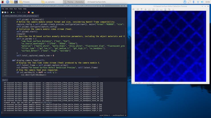
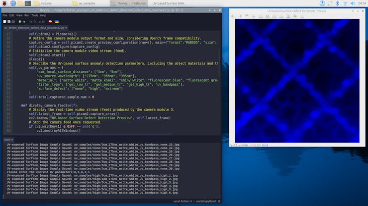
🖥️ Real-time video stream on Raspberry Pi 4 while collecting image samples

 

 

 

Circular Conveyor - Step 0: Migrating project from Raspberry Pi 4 to Raspberry Pi 5 to utilize two different camera module 3 versions (regular Wide and NoIR Wide) simultaneously

After successfully concluding my experiments with the data collection rig and constructing the UV-applied plastic surface image dataset with enough discrepancy (contrast) to train a visual anomaly detection model, I started to work on developing the industrial-grade proof-of-concept circular conveyor mechanism to explore different aspects of utilizing the substantial data I was collecting in a real-world manufacturing setting.

After training and building my FOMO-AD (visual anomaly detection model) on Edge Impulse Studio successfully — the training process is explained in the following step — I came to the conclusion that utilizing only the camera module with which I constructed my dataset was not applicable for a real-world scenario since camera types and attributes differ in manufacturing settings. Thus, to review my visual anomaly detection model's behaviour with image samples generated by a different camera type, I decided to add a secondary camera to my mechanism. As the secondary camera, I selected the NoIR version of the Raspberry Pi camera module 3, which is based on the same IMX708 image sensor but has no integrated IR filter, producing distinctly different UV-induced image samples than the regular Wide module, but with the same procedure.

In this regard, I decided to migrate my project from the Raspberry Pi 4 to the Raspberry Pi 5 since I wanted to capitalize on the Pi 5’s dual-CSI ports, which allowed me to utilize two different types of camera modules (regular Wide and NoIR Wide) simultaneously and develop a feature-rich industrial-grade surface defect detection mechanism employing a regular camera and a night-vision camera.

#️⃣ Similar to the Raspberry Pi 4, after setting up the Raspberry Pi OS on the Raspberry Pi 5 via the Raspberry Pi Imager, I installed the required Python modules (libraries) to continue developing.

sudo apt-get update

sudo apt-get install python3-opencv

#️⃣ Contrary to the Raspberry Pi 4, the dual CSI ports of the Raspberry Pi 5 are not compatible with FFC cables. Thus, I purchased official FPC connector cables (300 mm and 500 mm) to attach the regular Wide and the NoIR Wide camera modules to the respective CSI ports.

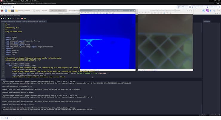
#️⃣ Before proceeding with developing my circular conveyor mechanism with the dual camera setup, I needed to establish the workflow for running both cameras simultaneously. Thus, I decided to modify my previous Python script for capturing UV-applied plastic surface image samples with the camera module 3 Wide.

Even though I programmed the Raspberry Pi 5 to capture image samples produced by two different camera modules simultaneously, I did not expand my dataset or retrain the model with images generated by the camera module 3 NoIR Wide, as I wanted to study my model's behaviour while running inferences in a different manufacturing setting.

📁 uv_defect_detection_collect_data_w_rasp_5_camera_mod_wide_and_noir.py

⭐ Include the required system and third-party libraries.

⭐ Uncomment to modify the libcamera log level to bypass the libcamera warnings if you want clean shell messages while entering user inputs.

import cv2
from picamera2 import Picamera2, Preview
from time import sleep
from threading import Thread

# Uncomment to disable libcamera warnings while collecting data.
#import os
#os.environ["LIBCAMERA_LOG_LEVELS"] = "4"

#️⃣ To bundle all the functions to write a more concise script, I used a Python class.

⭐ In the __init__ function:

⭐ Define a picamera2 object addressing the CSI port of the Raspberry Pi camera module 3 Wide.

⭐ Define the output format and size (resolution) of the images captured by the regular camera module 3 to obtain an OpenCV-compatible buffer — RGB888. Then, configure the picamera2 object accordingly.

⭐ Initialize the video stream (feed) produced by the regular camera module 3.

⭐ Define a secondary picamera2 object addressing the CSI port of the Raspberry Pi camera module 3 NoIR Wide.

⭐ Define the output format and size (resolution) of the images captured by the camera module 3 NoIR to obtain an OpenCV-compatible buffer — RGB888. Then, configure the picamera2 object accordingly.

⭐ Initialize the video stream (feed) produced by the camera module 3 NoIR.

⭐ Describe all possible experiment parameters in a Python dictionary for easy access.

⭐ Define the camera attributes and respective total sample numbers for the concurrent data collection process.

class uv_defect_detection():
    def __init__(self):
        # Define the Picamera2 object for communicating with the Raspberry Pi camera module 3 Wide.
        self.cam_wide = Picamera2(0)
        # Define the camera module frame output format and size, considering OpenCV frame compatibility.
        capture_config = self.cam_wide.create_preview_configuration(raw={}, main={"format":"RGB888", "size":(640,640)})
        self.cam_wide.configure(capture_config)
        # Initialize the camera module continuous video stream (feed).
        self.cam_wide.start()
        sleep(2)
        
        # Define the Picamera2 object for communicating with the Raspberry Pi camera module 3 NoIR Wide.
        self.cam_noir_wide = Picamera2(1)
        # Define the camera module NoIR frame output format and size, considering OpenCV frame compatibility.
        capture_config_noir = self.cam_wide.create_preview_configuration(raw={}, main={"format":"RGB888", "size":(640,640)})
        self.cam_noir_wide.configure(capture_config_noir)
        # Initialize the camera module NoIR continuous video stream (feed).
        self.cam_noir_wide.start()
        sleep(2)
        
        # Describe the surface anomaly detection conditions based on UV-exposure, including plastic material types, applied UV wavelengths, and the employed camera filter categories.
        self.uv_params = {
            "cam_focal_surface_distance": ["3cm", "5cm"],
            "uv_source_wavelength": ["275nm", "365nm", "395nm"],
            "material": ["matte_white", "matte_khaki", "shiny_white", "fluorescent_blue", "fluorescent_green"],
            "filter_type": ["gel_low_tr", "gel_medium_tr", "gel_high_tr", "uv_bandpass"],
            "surface_defect": ["none", "high", "extreme"]           
        }
        
        # Define the required camera information for the data collection process.
        self.active_cam_info = [{"name": "wide", "total_captured_sample_num": 0}, {"name": "wide_noir", "total_captured_sample_num": 0}]
        
		...

⭐ In the display_camera_feeds function:

⭐ Obtain the latest frame generated by the regular camera module 3.

⭐ Show the obtained frame on the screen via the built-in OpenCV tools.

⭐ Then, obtain the latest frame produced by the camera module 3 NoIR and show the retrieved frame in a separate window on the screen via the built-in OpenCV tools.

⭐ Stop both camera feeds (regular Wide and NoIR Wide) and terminate individual OpenCV windows once requested.

def display_camera_feeds(self):
        # Display the real-time video stream (feed) produced by the camera module 3 Wide.
        self.latest_frame_wide = self.cam_wide.capture_array()
        cv2.imshow("UV-based Surface Defect Detection [Wide Preview]", self.latest_frame_wide)
        # Display the real-time video stream (feed) produced by the camera module 3 NoIR Wide.
        self.latest_frame_noir = self.cam_noir_wide.capture_array()
        cv2.imshow("UV-based Surface Defect Detection [NoIR Preview]", self.latest_frame_noir)            
        # Stop all camera feeds once requested.
        if cv2.waitKey(1) & 0xFF == ord('q'):
            cv2.destroyAllWindows()
            self.cam_wide.stop()
            self.cam_wide.close()
            print("\nWide Camera Feed Stopped\n")
            self.cam_noir_wide.stop()
            self.cam_noir_wide.close()
            print("\nWide NoIR Camera Feed Stopped!\n")

⭐ In the camera_feeds function, initiate the loop to show the latest frames produced by the regular Wide and NoIR Wide camera modules consecutively to observe the real-time video streams (feeds) simultaneously.

def camera_feeds(self):
        # Start the camera video streams (feeds) in a loop.
        while True:
            self.display_camera_feeds()

⭐ In the save_uv_img_samples function:

⭐ Define the file name and path of the current image sample by applying the passed experiment parameters.

⭐ The given parameters also determine whether the latest frame should be obtained from the regular camera module or the NoIR camera module.

⭐ Up to the passed batch number, save the latest successive frames generated by the selected camera module (regular or NoIR) with the given file name and path, differentiated by the sample number.

⭐ Wait half a second before obtaining the next available frame.

def save_uv_img_samples(self, params, batch):
        # Based on the provided UV-based anomaly detection conditions and the selected camera type, generate the given image sample path and partial file name.
        selected_cam = self.active_cam_info[int(params[5])]["name"]
        img_file = "uv_samples/{}/{}/{}_{}_{}_{}_{}".format(
                                                             selected_cam,
                                                             self.uv_params["surface_defect"][int(params[4])],
                                                             self.uv_params["cam_focal_surface_distance"][int(params[0])],
                                                             self.uv_params["uv_source_wavelength"][int(params[1])],
                                                             self.uv_params["material"][int(params[2])],
                                                             self.uv_params["filter_type"][int(params[3])],
                                                             self.uv_params["surface_defect"][int(params[4])]
                                                         )
        
        # Save the latest frames captured by the selected camera type — the camera module 3 Wide or the camera module 3 NoIR Wide — consecutively according to the passed batch number.
        for i in range(batch):
            self.active_cam_info[int(params[5])]["total_captured_sample_num"] += 1
            if (self.active_cam_info[int(params[5])]["total_captured_sample_num"] > 30): self.active_cam_info[int(params[5])]["total_captured_sample_num"] = 1
            _img_file = img_file + "_{}.jpg".format(self.active_cam_info[int(params[5])]["total_captured_sample_num"])
            if(selected_cam == "wide"):
                cv2.imwrite(_img_file, self.latest_frame_wide)
            elif(selected_cam == "wide_noir"):
                cv2.imwrite(_img_file, self.latest_frame_noir)                
            # Wait before getting the next available frame.
            sleep(0.5)
            print("UV-exposed Surface Image Sample Saved [" + selected_cam + "]: " + _img_file)

⭐ In the obtain_and_decode_input function:

⭐ Initiate the loop to obtain user inputs continuously.

⭐ Once the user input is fetched, decode the retrieved string to obtain the given experiment parameters as an array. Then, check the number of the extracted experiment parameters.

⭐ If matched, capture image samples up to the given batch number (10) with the selected camera module and record the given experiment parameters to the sample file names.

def obtain_and_decode_input(self):
        # Initiate the user input prompt to obtain the given UV-exposure conditions for the data collection process.
        while True:
            passed_params = input("Please enter the current UV-exposure conditions:")
            # Decode the passed string to extract the provided parameters.
            decoded_params = passed_params.split(",")
            # Check the number of the extracted parameters.
            if (len(decoded_params) == 6):
                # If matched, capture image samples according to the passed batch number — 10.
                self.save_uv_img_samples(decoded_params, 10)
            else:
                print("Incorrect parameter number!")

#️⃣ As the built-in Python input function needs to check for new user input without interruptions, it cannot run with the real-time video streams generated by OpenCV in the same operation (runtime), which processes the latest frames produced by the regular Wide and NoIR Wide camera modules continuously. Therefore, I utilized the built-in Python threading module to run multiple operations concurrently and synchronize them.

⭐ Define the uv_defect_detection class object.

⭐ Declare and initialize a Python thread for running the real-time video streams (feeds) produced by the regular camera module 3 and the camera module 3 NoIR.

⭐ Outside of the video streams operation (thread), check new user inputs continuously to obtain the provided experiment parameters.

uv_defect_detection_obj = uv_defect_detection()

# Declare and initialize a Python thread for the camera module 3 Wide and the camera module 3 NoIR Wide video streams (feeds).
Thread(target=uv_defect_detection_obj.camera_feeds).start()

# Obtain the provided UV-exposure conditions as user input continuously.
uv_defect_detection_obj.obtain_and_decode_input()

 

 

 

Circular Conveyor - Step 1: Building a visual anomaly detection model (FOMO-AD) w/ Edge Impulse Enterprise

Since Edge Impulse provides developer-friendly tools for advanced AI applications and supports almost every development board due to its model deployment options, I decided to utilize Edge Impulse Enterprise to build my visual anomaly detection model. Also, Edge Impulse Enterprise incorporates elaborate model architectures for advanced computer vision applications and optimizes the state-of-the-art vision models for edge devices and single-board computers such as the Raspberry Pi 5.

Among the diverse machine learning algorithms provided by Edge Impulse, I decided to employ FOMO-AD (visual anomaly detection), which is specifically developed for handling unseen data, like defects in a product during manufacturing.

While labeling the UV-applied plastic surface image samples, I needed to utilize the default classes required by Edge Impulse to enable the F1 score calculation:

• no anomaly
• anomaly

Plausibly, Edge Impulse Enterprise enables developers with advanced tools to build, optimize, and deploy each available machine learning algorithm as supported firmware for nearly any device you can think of. Therefore, after training and validating, I was able to deploy my FOMO-AD model as an EIM binary for Linux (AARCH64) compatible with Raspberry Pi 5.

To utilize the advanced AI tools provided by Edge Impulse, you can register here.

Furthermore, you can inspect this FOMO-AD visual anomaly detection model on Edge Impulse as a public project.

 

 

 

 

Circular Conveyor - Step 1.1: Uploading and labeling the UV-applied plastic surface image samples

#️⃣ First, I created a new project on my Edge Impulse Enterprise account.

#️⃣ To label image samples manually for FOMO-AD visual anomaly detection models, go to Dashboard ➡ Project info ➡ Labeling method and select One label per data item.

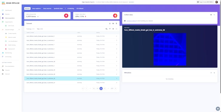
#️⃣ To upload training and testing UV-applied plastic surface image samples as individual files, I opened the Data acquisition section and clicked the Upload data icon.

#️⃣ I utilized default Edge Impulse configurations to distinguish training and testing image samples to enable the F1 score calculation.

#️⃣ For training samples, I selected the Training category and entered no anomaly as their shared label.

#️⃣ For testing samples, I selected the Testing category and entered anomaly as their shared label.

As I wanted this visual anomaly detection model to represent all of my experiments, I uploaded all image samples with the none surface defect stage as the training samples and all image samples with the extreme surface defect stage as the testing samples.

• /none (3600 samples)
• /extreme (3600 samples)

 

 

 

Circular Conveyor - Step 1.2: Training the FOMO-AD (visual anomaly detection) model

An impulse (an application developed and optimized by Edge Impulse) takes raw data, applies signal processing to extract features, and then utilizes a learning block to classify new data.

For my application, I created the impulse by employing the Image processing block and the Visual Anomaly Detection - FOMO-AD learning block.

Image processing block processes the passed raw image input as grayscale or RGB (optional) to produce a reliable features array.

FOMO-AD learning block represents the officially supported machine learning algorithms, based on a selectable backbone for feature extraction and a scoring function (PatchCore, GMM anomaly detection).

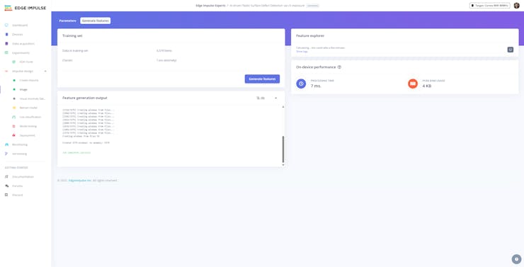
#️⃣ First, I opened the Impulse design ➡ Create impulse section, set the model image resolution to 320 x 320, and selected the Fit shortest axis resize mode so as to scale (resize) the given image samples precisely. To complete the impulse creation, I clicked Save Impulse.

#️⃣ To modify the raw image features in the applicable format, I navigated to the Impulse design ➡ Image section, set the Color depth parameter as RGB, and clicked Save parameters.

#️⃣ Then, I proceeded to click Generate features to extract the required features for training by applying the Image processing block.

#️⃣ After extracting features successfully, I navigated to the Impulse design ➡ Visual Anomaly Detection section and modified the neural network settings and architecture to achieve reliable accuracy and validity.

#️⃣ First, I selected the Training processor as GPU since I uploaded an extensive dataset providing more than 3000 training image samples.

#️⃣ According to my prolonged experiments, I assigned the final model settings as follows.

📌 Training settings:

• Training processor ➡ GPU
• Capacity ➡ High

📌 Neural network architecture:

• MobileNetV2 0.35
• Gaussian Mixture Model (GMM)

#️⃣ Adjusting Capacity higher means a higher number of (Gaussian) components, making the visual anomaly detection model more adapted to the original distribution.

#️⃣ After training the model with the final configurations, Edge Impulse did not evaluate the F1 score (accuracy) due to the nature of the visual anomaly model training process.

 

 

 

Circular Conveyor - Step 1.3: Evaluating the model accuracy and deploying the validated model

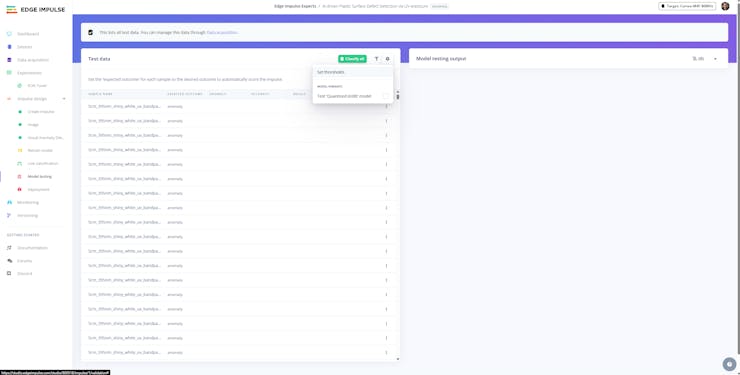
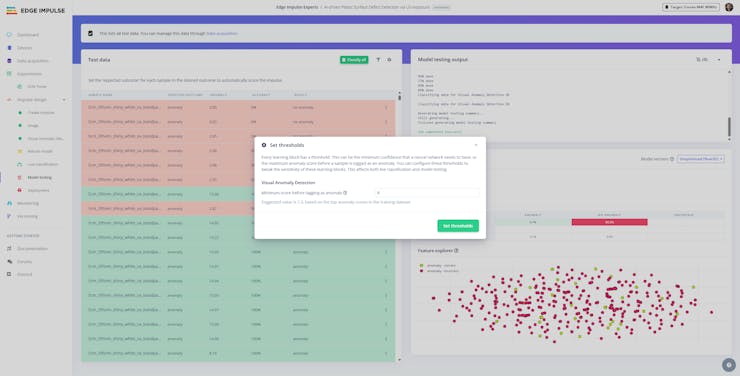
Testing the FOMO-AD visual anomaly detection models is extremely salient for getting precise results while running inferences on the device. In addition to evaluating the F1 precision score (accuracy), Edge Impulse allows the user to tweak the learning block sensitivity by adjusting the anomaly (confidence) threshold, resulting in a much more adaptable model for real-world operations.

#️⃣ First, to obtain the validation score of the trained model based on the provided testing samples, I navigated to the Impulse design ➡ Model testing section and clicked Classify all.

#️⃣ Based on the initial F1 score, I started to rigorously experiment with different model variants and anomaly (confidence) thresholds to pinpoint the optimum settings for the real-world conditions.

#️⃣ Although Edge Impulse suggested 7.3 as the confidence threshold based on the top anomaly scores in the training dataset, it performed poorly for the Unoptimized (float32) model variant. According to my experiments, I found out that a 2.12 confidence threshold is the sweet spot for the unoptimized version, leading to an 83.74% F1 score (accuracy).

#️⃣ On the other hand, the Quantized (int8) model variant performed best with an 8 confidence threshold, leading to a 100% F1 score (accuracy).

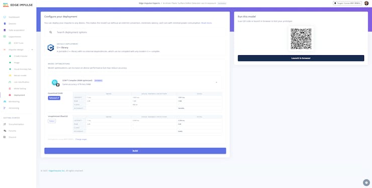
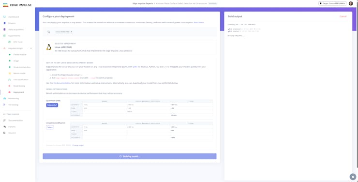
#️⃣ To deploy the validated model optimized for my hardware, I navigated to the Impulse design ➡ Deployment section and searched for Linux(AARCH64).

#️⃣ I chose the Quantized (int8) model variant (optimization) to achieve the optimal performance while running the deployed model.

#️⃣ Finally, I clicked Build to download the produced EIM binary, containing the trained visual anomaly detection model.

 

 

 

Circular Conveyor - Step 2: Setting up Apache web server with MariaDB database and Edge Impulse Linux Python SDK on Raspberry Pi 5

As mentioned earlier, I decided to develop a web dashboard for the circular conveyor mechanism and host it locally on the Raspberry Pi 5. Thus, I decided to utilize Apache as the local server for my web dashboard, providing all necessary tools to build a full-fledged PHP-based application.

To easily access and run my FOMO-AD visual anomaly detection model (EIM binary) via a Python script, I also installed the Edge Impulse Linux Python SDK on the Raspberry Pi 5.

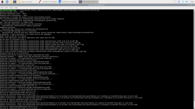
#️⃣ First, I installed the Apache web server with a MariaDB database, the PHP MySQL package, and the PHP cURL package via the terminal.

sudo apt-get install apache2 php mariadb-server php-mysql php-curl -y

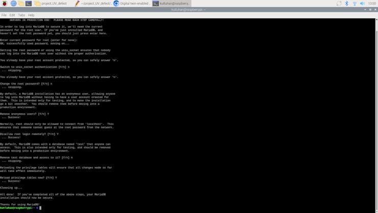
#️⃣ To utilize the MariaDB database, I set the root user by strictly following the secure installation prompt.

sudo mysql_secure_installation

#️⃣ After setting up the Apache server, I proceeded to install the official Edge Impulse Python SDK with all dependencies.

sudo apt-get install libatlas-base-dev libportaudio2 libportaudiocpp0 portaudio19-dev python3-pip

sudo pip3 install pyaudio edge_impulse_linux --break-system-packages

#️⃣ Since I did not create a virtual environment, I needed to utilize the break-system-packages command-line argument to bypass the system-wide package installation error.

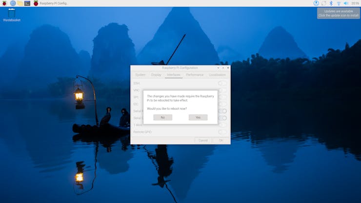
As discussed earlier, I decided to design a unique controller board (PCB) for the circular conveyor mechanism in the form of a Raspberry Pi 5 shield (hat). Since the controller board would be based on an ATmega328P, I decided to establish the data transfer via serial communication. In this regard, before prototyping the circular conveyor interface, I needed to enable the UART serial communication protocol on the Raspberry Pi 5.

#️⃣ To activate the UART serial communication via GPIO pins, I enabled the Serial Port interface on Raspberry Pi Configuration. Then, I rebooted the Pi 5.

 

 

 

Circular Conveyor - Step 3: Prototyping and initial programming of the circular conveyor interface with Arduino Uno

Before proceeding with developing the mechanical parts and the controller board (interface) of the circular conveyor mechanism, I needed to ensure that every sensor and component was operating as anticipated. In this regard, I decided to utilize an Arduino Uno to prototype the circular conveyor interface. Since I had an original Arduino Uno, which is based on the ATmega328P, I was able to test and run my initial programming of the conveyor interface effortlessly.

#️⃣ As I decided to design two conveyor drivers sharing the load while rotating the conveyor chain, I utilized two Nema 17 (17HS3401) stepper motors controlled by two separate A4988 driver modules.

#️⃣ Since I wanted to utilize neodymium magnets to align the center of the plastic object surfaces held by the plastic object carriers of the circular conveyor with the focal points of both camera modules (regular Wide and NoIR Wide), I used two magnetic Hall-effect sensor modules (KY-003).

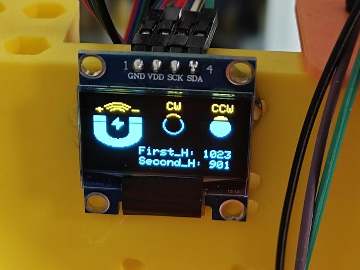
#️⃣ To provide the user with a feature-rich interface, I connected an SSD1306 OLED display and four control buttons.

#️⃣ To enable the user to adjust the conveyor attributes manually, I added two long-shaft potentiometers.

#️⃣ Since I needed to supply power for a lot of current-demanding electronic components with different operating voltages, I decided to convert my old ATX power supply unit (PSU) into a simple bench power supply by utilizing an ATX adapter board (XH-M229) providing stable 3.3V, 5V, and 12V. For each power output of the adapter board, I soldered wires to attach a DC-barrel-to-wire jack (male) in order to create a production-ready bench power supply.

#️⃣ Furthermore, as a part of my initial programming experiments, I reviewed the data transmission between the software serial port of the Arduino Uno and the hardware UART serial port (GPIO) of the Raspberry Pi 5.

#️⃣ Since Arduino Uno and ATmega328P operate at 5V while Raspberry Pi 5 requires 3.3V logic level voltage, their GPIO pins cannot be connected directly, even for serial communication. Therefore, I utilized a bi-directional logic level converter to shift the voltage between the respective pin connections.

 

 

 

Circular Conveyor - Step 3.1: Setting up and configuring ATMEGA328P-PU as an Arduino Uno

After completing my initial Arduino Uno prototyping and programming, I started to set up my ATmega328P-PU to be able to move electrical components from the Arduino Uno to its corresponding pins to continue developing the circular conveyor interface.

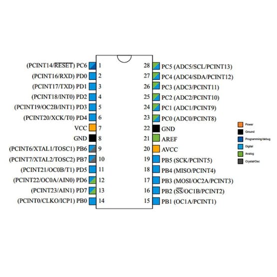
#️⃣ First, based on the ATmega328P datasheet, I built the required circuitry to drive the ATmega328P single-chip microcontroller, consisting of these electrical components:

• 16.000 MHz crystal [1]
• 10K resistor [1]
• 22pF ceramic disc capacitor [2]
• 10uF 250v electrolytic capacitor [1]

#️⃣ Since I did not want to add an onboard USB port to my PCB, I decided to upload code files to the ATmega328P via an external FTDI adapter (programming board), which requires an additional 100nF ceramic disc capacitor while connecting its DTR/RTS pin to the reset pin of the ATmega328P.

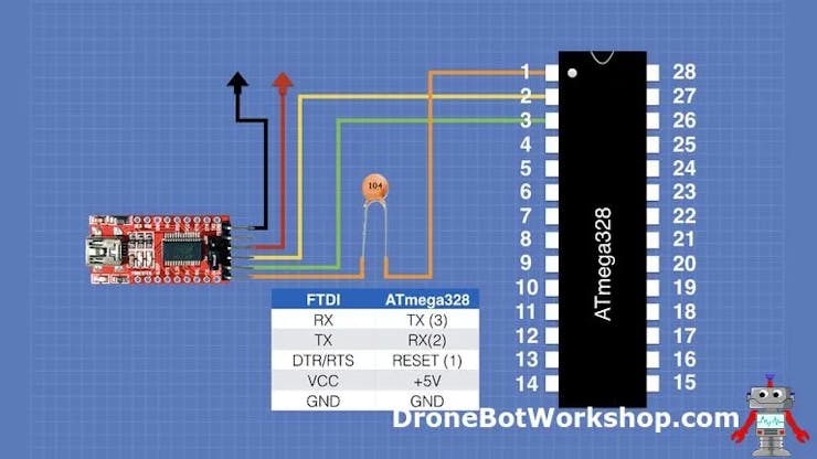
📌 DroneBot Workshop provided in-depth written and video tutorials regarding utilizing the ATmega328P and the FTDI adapter, from which I got the connection schematics above. So, please refer to DroneBot Workshop's tutorial to get more information about the ATmega328P microcontroller.

Since I wanted to program the ATmega328P as an Arduino Uno via the Arduino IDE, I purchased ATmega328P-PU chips, which come with the preloaded (burned) Arduino bootloader in their EEPROM. Nonetheless, any of my ATmega328P chips with the PU version had been recognized by the latest version of Arduino IDE — 2.3.6.

Therefore, I needed to burn the required bootloader manually to my ATmega328P-PU by employing a different Arduino Uno, other than the one I used to prototype the conveyor interface, as an in-system program (ISP), as depicted in this official Arduino guideline.

#️⃣ First, I connected the Arduino Uno to the computer and selected its COM port on the Arduino IDE.

#️⃣ Then, I navigated to File ➡ Examples ➡ ArduinoISP and uploaded the ArduinoISP example to the Arduino UNO.

#️⃣ Since the ISP example uses the SPI protocol to burn the bootloader, I connected the hardware SPI pins (MISO, MOSI, and SCK) of the Arduino Uno to the corresponding SPI pins of the ATmega328P.

#️⃣ I also connected pin 10 to the ATmega328P reset pin since the ISP example uses D10 to reset the target microcontroller, rather than the SS pin.

• MOSI (D11) ➡ 17
• MISO (D12) ➡ 18
• SCK (D13) ➡ 19
• D10 ➡ 1

#️⃣ After connecting the Arduino Uno SPI pins to the ATmega328P SPI pins, I selected Tools ➡ Programmer ➡ Arduino as ISP. Then, I selected the board as Arduino Uno since I wanted to burn the Arduino Uno bootloader to the target ATmega328P chip.

#️⃣ After configuring bootloader settings, I clicked Tools ➡ Burn Bootloader to initiate the bootloader burning procedure.

#️⃣ After burning the Arduino Uno bootloader to my ATmega328P chip successfully, I uploaded a simple program via the external FTDI adapter to test whether the ATmega328P chip behaves as an Arduino Uno.

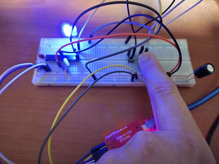
#️⃣ Once I confirmed the ATmega328P worked as an Arduino Uno, I connected a button to its reset pin and GND in order to restart my program effortlessly in case of logic errors.

#️⃣ Finally, I migrated all of the electrical components to the ATmega328P, considering its pin names equivalent to the Arduino Uno's.

// Connections
// ATMEGA328P-PU :  
//                                Nema 17 (17HS3401) Stepper Motor w/ A4988 Driver Module [Motor 1]
// 5V      ------------------------ VDD
// GND     ------------------------ GND
// D2      ------------------------ DIR
// D3      ------------------------ STEP
//                                Nema 17 (17HS3401) Stepper Motor w/ A4988 Driver Module [Motor 2]
// 5V      ------------------------ VDD
// GND     ------------------------ GND
// D4      ------------------------ DIR
// D5      ------------------------ STEP
//                                SSD1306 OLED Display (128x64)
// 5V      ------------------------ VCC
// GND     ------------------------ GND
// A4      ------------------------ SDA
// A5      ------------------------ SCL
//                                Raspberry Pi 5 
// D6 (RX) ------------------------ GPIO 14 (TXD)
// D7 (TX) ------------------------ GPIO 15 (RXD)
//                                Magnetic Hall Effect Sensor Module (KY-003) [First] 
// GND     ------------------------ -
// 5V      ------------------------ +
// A0      ------------------------ S
//                                Magnetic Hall Effect Sensor Module (KY-003) [Second] 
// GND     ------------------------ -
// 5V      ------------------------ +
// A1      ------------------------ S
//                                Long-shaft B4K7 Potentiometer (Speed) 
// A2      ------------------------ Signal
//                                Long-shaft B4K7 Potentiometer (Station) 
// A3      ------------------------ Signal
//                                Control Button (A)
// D8      ------------------------ +
//                                Control Button (B)
// D9      ------------------------ +
//                                Control Button (C)
// D10     ------------------------ +
//                                Control Button (D)
// D11     ------------------------ +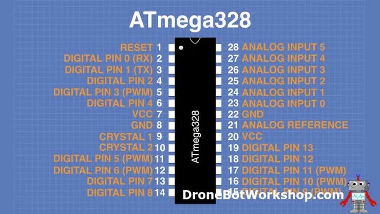

 

 

 

Circular Conveyor - Step 4: Programming ATMEGA328P-PU as the circular conveyor interface

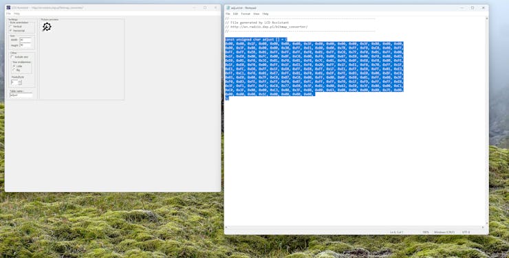
To prepare monochromatic images in order to display custom logos on the SSD1306 OLED screen, I followed this process.

#️⃣ First, I converted monochromatic bitmaps to compatible C data arrays by utilizing LCD Assistant.

#️⃣ Based on the SSD1306 screen type, I selected the Horizontal byte orientation.

#️⃣ After converting all logos successfully, I created a header file — logo.h — to store them.

#️⃣ I installed the libraries required to control the attached electronic components:

📚 SoftwareSerial (built-in) | Inspect

📚 Adafruit_SSD1306 | Download

📚 Adafruit-GFX-Library | Download

📁 ai_driven_surface_defect_detection_circular_sprocket_conveyor.ino

⭐ Include the required libraries.

#include <SoftwareSerial.h>
#include <Adafruit_GFX.h>
#include <Adafruit_SSD1306.h>

⭐ Import custom logos (C data arrays).

#include "logo.h"

⭐ Declare a software serial port to communicate with Raspberry Pi 5.

SoftwareSerial rasp_pi_5 (6, 7); // RX, TX

⭐ Define the SSD1306 display configurations and declare the SSD1306 class instance.

#define SCREEN_WIDTH 128 // OLED display width, in pixels
#define SCREEN_HEIGHT 64 // OLED display height, in pixels
#define OLED_RESET    -1 // Reset pin # (or -1 if sharing Arduino reset pin)
Adafruit_SSD1306 display(SCREEN_WIDTH, SCREEN_HEIGHT, &Wire, OLED_RESET);

⭐ Define the analog pins for the Hall-effect sensor modules (KY-003).

#define first_hall_effect_sensor    A0
#define second_hall_effect_sensor   A1

⭐ Define the digital pins for the control buttons.

#define control_button_A   8
#define control_button_B   9
#define control_button_C   10
#define control_button_D   11

⭐ Declare all of the variables required by the circular conveyor drivers by creating a struct.

struct stepper_config{
  #define m_num 2
  int _pins[m_num][2] = {{2, 3}, {4, 5}}; // (DIR, STEP)
  // Assign the required revolution and initial speed variables based on drive sprocket conditions.
  int stepsPerRevolution = 200;
  int sprocket_speed = 12000;
  // Assign stepper motor tasks based on the associated part.
  int sprocket_1 = 0, sprocket_2 = 1;  
  // Declare the circular conveyor station pending time for each inference session.
  int station_pending_time = 5000;
  // Define the necessary potentiometer configurations for adjusting the sprocket speed and the station pending time.
  int pot_speed_pin = A2, pot_speed_min = 8000, pot_speed_max = 25000;
  int pot_pending_pin = A3, pot_pending_min = 3000, pot_pending_max = 30000;
};

⭐ Initiate the declared software serial port with its assigned RX and TX pins to start the data transmission process with the Raspberry Pi 5.

rasp_pi_5.begin(9600);

⭐ Activate the assigned DIR and STEP pins connected to the A4988 driver modules, controlling the Nema 17 stepper motors.

for(int i = 0; i < m_num; i++){ pinMode(stepper_config._pins[i][0], OUTPUT); pinMode(stepper_config._pins[i][1], OUTPUT); }

⭐ Initialize the SSD1306 class instance.

display.begin(SSD1306_SWITCHCAPVCC, 0x3C);
  display.display();
  delay(1000);

⭐ In the show_screen function, program different screen layouts (interfaces) based on the ongoing conveyor operation, the given user commands, and the real-time sensor readings.

void show_screen(char _type, int _opt){
  // According to the given parameters, show the requested screen type on the SSD1306 OLED screen.
  int str_x = 5, str_y = 5;
  int l_h = 8, l_sp = 5;
  if(_type == 'h'){
    display.clearDisplay();
    switch(_opt){
      case 0: display.drawBitmap(str_x, str_y, home_bits, home_w, home_h, SSD1306_WHITE); break;
      case 1: display.drawBitmap(str_x, str_y, adjust_bits, adjust_w, adjust_h, SSD1306_WHITE); break;
      case 2: display.drawBitmap(str_x, str_y, check_bits, check_w, check_h, SSD1306_WHITE); break;
      case 3: display.drawBitmap(str_x, str_y, serial_bits, serial_w, serial_h, SSD1306_WHITE); break;
      case 4: display.drawBitmap(str_x, str_y, activate_bits, activate_w, activate_h, SSD1306_WHITE); break;
    }
    display.setTextSize(1);
    (_opt == 1) ? display.setTextColor(SSD1306_BLACK, SSD1306_WHITE) : display.setTextColor(SSD1306_WHITE);
    display.setCursor((SCREEN_WIDTH/2)-str_x, str_y);
    display.print("1. Adjust");
    str_y += 2*l_h;
    (_opt == 2) ? display.setTextColor(SSD1306_BLACK, SSD1306_WHITE) : display.setTextColor(SSD1306_WHITE);
    display.setCursor((SCREEN_WIDTH/2)-str_x, str_y);
    display.print("2. Check");
    str_y += 2*l_h;
    (_opt == 3) ? display.setTextColor(SSD1306_BLACK, SSD1306_WHITE) : display.setTextColor(SSD1306_WHITE);
    display.setCursor((SCREEN_WIDTH/2)-str_x, str_y);
    display.print("3. Serial");
    str_y += 2*l_h;
    (_opt == 4) ? display.setTextColor(SSD1306_BLACK, SSD1306_WHITE) : display.setTextColor(SSD1306_WHITE);
    display.setCursor((SCREEN_WIDTH/2)-str_x, str_y);
    display.print("4. Activate");
    display.display();
    delay(500);
  }
  if(_type == 'a'){
    int rect_w = l_h, rect_h = l_h;
    display.clearDisplay();
    display.drawBitmap(str_x, str_y, adjust_bits, adjust_w, adjust_h, SSD1306_WHITE);
    display.setTextSize(1);
    display.setTextColor(SSD1306_WHITE);
    str_x = (SCREEN_WIDTH/2);
    display.fillRect(str_x-rect_w-l_sp, str_y+(l_h/2)-(rect_h/2), rect_w, rect_h, SSD1306_WHITE);
    display.setCursor(str_x, str_y);
    display.print("Speed:");
    str_x += 5*l_sp;
    str_y += l_h;
    display.setCursor(str_x, str_y);
    display.print(current_pot_speed_value);
    str_y += l_h;
    display.setCursor(str_x, str_y);
    display.setTextColor(SSD1306_BLACK, SSD1306_WHITE);
    display.print(stepper_config.sprocket_speed);
    str_x -= 5*l_sp;
    str_y += 2*l_h;
    display.setTextColor(SSD1306_WHITE);
    display.setCursor(str_x, str_y);
    display.fillRect(str_x-rect_w-l_sp, str_y+(l_h/2)-(rect_h/2), rect_w, rect_h, SSD1306_WHITE);
    display.print("Pending:");
    str_x += 5*l_sp;
    str_y += l_h;
    display.setCursor(str_x, str_y);
    display.print(current_pot_pending_value);
    str_y += l_h;
    display.setCursor(str_x, str_y);
    display.setTextColor(SSD1306_BLACK, SSD1306_WHITE);    
    display.print(stepper_config.station_pending_time);
    display.display();
  }
  if(_type == 'c'){
    int c_r = l_h;
    display.clearDisplay();
    display.drawBitmap(str_x, str_y, check_bits, check_w, check_h, SSD1306_WHITE);
    display.setTextSize(1);
    display.setTextColor(SSD1306_WHITE);
    str_x = (SCREEN_WIDTH-check_w-(4*c_r))/3;
    str_x = check_w + str_x + c_r + l_sp;
    str_y += 2*l_h;
    (!digitalRead(control_button_A)) ? display.fillCircle(str_x, str_y, c_r, SSD1306_WHITE) : display.drawCircle(str_x, str_y, c_r, SSD1306_WHITE);
    display.setCursor(str_x-(l_h/2)-1, l_sp/2);
    display.print("CW");
    str_x = SCREEN_WIDTH - c_r - (2*l_sp);
    (!digitalRead(control_button_C)) ? display.fillCircle(str_x, str_y, c_r, SSD1306_WHITE) : display.drawCircle(str_x, str_y, c_r, SSD1306_WHITE);
    display.setCursor(str_x-(2*l_h/3)-2, l_sp/2);
    display.print("CCW");
    str_x = (2*l_sp/3) + check_w;
    str_y += c_r + (3*l_sp);
    display.setCursor(str_x, str_y);
    display.print("First_H: "); display.print(analogRead(first_hall_effect_sensor));
    str_y += 2*l_sp;
    display.setCursor(str_x, str_y);
    display.print("Second_H: "); display.print(analogRead(second_hall_effect_sensor));
    display.display();     
  }
  if(_type == 's'){
    display.clearDisplay();
    display.drawBitmap(str_x, str_y, serial_bits, serial_w, serial_h, SSD1306_WHITE);
    display.setTextSize(1);
    display.setTextColor(SSD1306_WHITE);
    str_x += serial_w + 3*l_sp;
    display.setCursor(str_x, str_y);
    display.print("Serial");
    str_y += l_h;
    display.setCursor(str_x, str_y);
    display.print("Initiated!");
    str_y += 3*l_h;
    display.setCursor(str_x, str_y);
    display.print("Response: "); display.print(rasp_pi_5_res);
    display.display();
  }
  if(_type == 'r'){
    display.clearDisplay();
    str_x = (SCREEN_WIDTH-activate_w)/2;
    str_y = (SCREEN_HEIGHT-activate_h)/2;
    display.drawBitmap(str_x, str_y, activate_bits, activate_w, activate_h, SSD1306_WHITE);
    display.display();
  }
}

⭐In the rasp_pi_5_response function, wait until Raspberry Pi 5 successfully sends a response to the transmitted data packet via serial communication.

⭐Once the retrieved data packet is processed, halt the loop checking for the response data packets.

⭐If Raspberry Pi 5 does not send a response in the given timeframe (station pending time), terminate the loop as well.

⭐Finally, return the fetched response.

char rasp_pi_5_response(){
  char rasp_pi_response = 'n';
  int port_wait = 0;
  // Wait until Raspberry Pi 5 successfully sends a response to the transmitted data packet via serial communication.
  while(rasp_pi_5_ongoing_transmission){
    port_wait++;
    while(rasp_pi_5.available() > 0){
      rasp_pi_response = rasp_pi_5.read();
    }
    delay(500);
    // Halt the loop once Raspberry Pi 5 returns a data packet (response) or does not respond in the given timeframe (station pending time).
    if(rasp_pi_response != 'n' || port_wait > stepper_config.station_pending_time){
      rasp_pi_5_ongoing_transmission = false;
    }
  }
  // Then, return the retrieved response.
  delay(500);
  return rasp_pi_response;  
}

⭐ In the send_data_packet_to_rasp_pi_5 function, transfer the passed data packet to Raspberry Pi 5 via serial communication.

⭐ Suspend code flow until acquiring a response from Raspberry Pi 5.

void send_data_packet_to_rasp_pi_5(String _data){
  rasp_pi_5_res = 'o';
  // Send the passed data packet to Raspberry Pi 5 via serial communication.
  rasp_pi_5.println(_data);
  // Suspend code flow until getting a response from Raspberry Pi 5.
  rasp_pi_5_ongoing_transmission = true; rasp_pi_5_res = rasp_pi_5_response();
  delay(1000);
}

⭐ In the conveyor_move function, based on the passed direction and step number, rotate two stepper motors driving the sprockets simultaneously to move the conveyor chain precisely.

• Clockwise [CW]: rotate stepper motors in the same direction (right) at the same velocity.
• Counterclockwise [CCW]: rotate stepper motors in the same direction (left) at the same velocity.

void conveyor_move(int step_number, int acc, String _dir){
  /*
      Move the sprocket-driven circular conveyor stations by controlling the rotation of the associated stepper motors.
      Clockwise [CW]: rotate stepper motors in the same direction (right) at the same velocity.
      Counterclockwise [CCW]: rotate stepper motors in the same direction (left) at the same velocity.
  */

  if(_dir == "CW"){
    digitalWrite(stepper_config._pins[stepper_config.sprocket_1][0], HIGH);
    digitalWrite(stepper_config._pins[stepper_config.sprocket_2][0], HIGH);
  }
  if(_dir == "CCW"){
    digitalWrite(stepper_config._pins[stepper_config.sprocket_1][0], LOW);
    digitalWrite(stepper_config._pins[stepper_config.sprocket_2][0], LOW);
  }

  for(int i = 0; i < step_number; i++){
    digitalWrite(stepper_config._pins[stepper_config.sprocket_1][1], HIGH);
    digitalWrite(stepper_config._pins[stepper_config.sprocket_2][1], HIGH);
    delayMicroseconds(stepper_config.sprocket_speed/acc);
    digitalWrite(stepper_config._pins[stepper_config.sprocket_1][1], LOW);
    digitalWrite(stepper_config._pins[stepper_config.sprocket_2][1], LOW);
    delayMicroseconds(stepper_config.sprocket_speed/acc);
  }  
}

⭐ On the home screen, update the highlighted interface option once the control button A or C is pressed. In other words, move the cursor between interface options.

• [A] ➡ Down
• [C] ➡ Up

⭐ Activate the highlighted interface option once the control button B is pressed.

• [B] ➡ Activate (Select)

show_screen('h', highlighted_menu_opt);

  // Update the highlighted interface option if the control button A or the control button C is pressed.
  if(!digitalRead(control_button_A)){
    highlighted_menu_opt++;
    if(highlighted_menu_opt > 4) highlighted_menu_opt = 0;
    delay(1000);
  }

  if(!digitalRead(control_button_C)){
    highlighted_menu_opt--;
    if(highlighted_menu_opt < 0) highlighted_menu_opt = 4;
    delay(1000);
  }

  // Select the highlighted interface option if the control button B is pressed.
  if(!digitalRead(control_button_B) && highlighted_menu_opt > 0){
    active_menu_opt[highlighted_menu_opt-1] = true;
    delay(250);
  }

⭐ Once the Adjust interface option is activated:

⭐ Obtain the latest potentiometer values and map the retrieved values according to the given thresholds.

⭐ Once the control button A is pressed, declare the associated potentiometer value (mapped) as the speed parameter for controlling the speed of the stepper motors driving the sprockets while rotating them.

⭐ Once the control button C is pressed, declare the associated potentiometer value (mapped) as the station pending time parameter, which is the intermission to give camera modules time to focus before running an inference.

⭐ Inform the user of the real-time parameter adjustments (declarations) on the screen.

⭐ Return to the home screen if the control button D is pressed.

if(active_menu_opt[0]){
    show_screen('a', highlighted_menu_opt);
    while(active_menu_opt[0]){
      // Obtain the latest potentiometer values and map the retrieved values according to the given thresholds.
      current_pot_speed_value = constrain(map(analogRead(stepper_config.pot_speed_pin), 50, 850, stepper_config.pot_speed_min, stepper_config.pot_speed_max), stepper_config.pot_speed_min, stepper_config.pot_speed_max);
      current_pot_speed_value /= 1000; current_pot_speed_value *= 1000;
      current_pot_pending_value = constrain(map(analogRead(stepper_config.pot_pending_pin), 50, 850, stepper_config.pot_pending_min, stepper_config.pot_pending_max), stepper_config.pot_pending_min, stepper_config.pot_pending_max);
      current_pot_pending_value /= 1000; current_pot_pending_value *= 1000;
      // Once the control button A is pressed, declare the associated potentiometer value (mapped) as the new conveyor sprocket speed parameter.
      if(!digitalRead(control_button_A)){ stepper_config.sprocket_speed =  current_pot_speed_value; }
      // Once the control button C is pressed, declare the associated potentiometer value (mapped) as the new conveyor station pending time parameter.
      if(!digitalRead(control_button_C)){ stepper_config.station_pending_time =  current_pot_pending_value; }
      // Inform the user of the latest adjustments on the screen.
      show_screen('a', highlighted_menu_opt);
      // Return to the home screen if the control button D is pressed.
      if(!digitalRead(control_button_D)){ active_menu_opt[0] = false; delay(500); }
    }
  }

⭐ Once the Check interface option is activated:

⭐ Once the control button A is pressed, rotate the stepper motors driving sprockets one step clockwise simultaneously.

⭐ Once the control button C is pressed, rotate the stepper motors driving sprockets one step counterclockwise simultaneously.

⭐ Obtain the real-time magnetic Hall-effect sensor raw readings.

⭐ Inform the user of the ongoing stepper motor movement and the real-time sensor readings on the screen.

⭐ Return to the home screen if the control button D is pressed.

if(active_menu_opt[1]){
    show_screen('c', highlighted_menu_opt);
    while(active_menu_opt[1]){     
      // Once the control button A is pressed, rotate the drive sprockets one step clockwise.
      if(!digitalRead(control_button_A)){ conveyor_move(stepper_config.stepsPerRevolution, 10, "CW"); }
      // Once the control button C is pressed, rotate the drive sprockets one step counterclockwise.
      if(!digitalRead(control_button_C)){ conveyor_move(stepper_config.stepsPerRevolution, 10, "CCW"); }
      // Inform the user of the given sprocket direction and the latest magnetic Hall effect sensor readings on the screen immediately.
      show_screen('c', highlighted_menu_opt);       
      // Return to the home screen if the control button D is pressed.
      if(!digitalRead(control_button_D)){ active_menu_opt[1] = false; delay(500); }
    }
  }

⭐ Once the Serial interface option is activated:

⭐ Once the control button A is pressed, send the test command to Raspberry Pi 5 via serial communication to check the two-way data transmission status.

⭐ Once the control button C is pressed, send the run command to Raspberry Pi 5 via serial communication to manually run consecutive inferences (regular Wide and NoIR Wide) with the FOMO-AD visual anomaly detection model.

⭐ Inform the user of the received response (data packet) from Raspberry Pi 5.

⭐ Return to the home screen if the control button D is pressed.

if(active_menu_opt[2]){
    show_screen('s', highlighted_menu_opt);
    while(active_menu_opt[2]){
      // Once the control button A is pressed, send the test command to Raspberry Pi 5 via serial communication to check the connection status.
      if(!digitalRead(control_button_A)){ send_data_packet_to_rasp_pi_5("test"); }
      // Once the control button C is pressed, send the run command to Raspberry Pi 5 via serial communication to manually run an inference.
      if(!digitalRead(control_button_C)){ send_data_packet_to_rasp_pi_5("run"); }
      // Inform the user of the latest received data packets from Raspberry Pi 5.
      show_screen('s', highlighted_menu_opt); 
      // Return to the home screen if the control button D is pressed.
      if(!digitalRead(control_button_D)){ active_menu_opt[2] = false; rasp_pi_5_res = 'o'; delay(500); }
    }
  }

⭐ Once the Activate interface option is activated:

⭐ Initiate the stepper motors to rotate the sprockets simultaneously to move the chain of the circular conveyor continuously but steadily.

⭐ Once both of the magnetic Hall-effect sensors detect neodymium magnets attached to the bottom of the plastic object carriers simultaneously, stop the circular conveyor motion immediately.

⭐ Wait until the given intermission (station pending time) passes to give the camera modules time to focus on the plastic object surfaces.

⭐ Then, send the run command to Raspberry Pi 5 via serial communication to initiate an inference session automatically.

⭐ Once Raspberry Pi 5 sends the response denoting that the inference session with the provided Edge Impulse FOMO-AD visual anomaly detection model was successful, resume the circular conveyor motion.

⭐ After concluding the inference session, move the chain of the circular conveyor further to prevent Hall-effect sensors from detecting the same neodymium magnets, which would lead to running inferences with the same plastic objects.

⭐ Terminate the automatic conveyor operations and return to the home screen once the control button D is pressed.

if(active_menu_opt[3]){
    show_screen('r', highlighted_menu_opt);
    while(active_menu_opt[3]){
      // Initiate the circular conveyor to move the conveyor stations continuously but steadily.
      conveyor_move(stepper_config.stepsPerRevolution/2, 10, "CW");
      // Via the neodymium magnets attached to the bottom of the conveyor stations, detect when stations are passing above the associated magnetic Hall effect sensors.
      if(analogRead(first_hall_effect_sensor) < 150 || analogRead(second_hall_effect_sensor) < 150){
        // Then, stop the circular conveyor motion immediately.
        circular_conveyor_station_stop = true;
        while(circular_conveyor_station_stop){
          // To give the cameras attached to Raspberry Pi 5 time to focus, wait until the given station pending time passes.
          delay(stepper_config.station_pending_time);
          // Then, send the run command to Raspberry Pi 5 via serial communication to initiate the inference session.
          send_data_packet_to_rasp_pi_5("run");
          // Once Raspberry Pi 5 runs an inference successfully with the provided Edge Impulse FOMO-AD model, resume the circular conveyor motion.
          if(rasp_pi_5_res == 's'){
            circular_conveyor_station_stop = false;
            station_magnet_detected = true;
            rasp_pi_5_res = 'o';
          }
        }
      }
      // After successfully completing the inference session and continuing the conveyor motion, rotate the drive sprockets additionally to prevent detecting the same station magnets consecutively.
      if(station_magnet_detected){
        conveyor_move(5*stepper_config.stepsPerRevolution, 10, "CW");
        station_magnet_detected = false;
      }
      // Return to the home screen if the control button D is pressed.
      if(!digitalRead(control_button_D)){ active_menu_opt[3] = false; delay(500); }
    }
  }

 

 

 

 

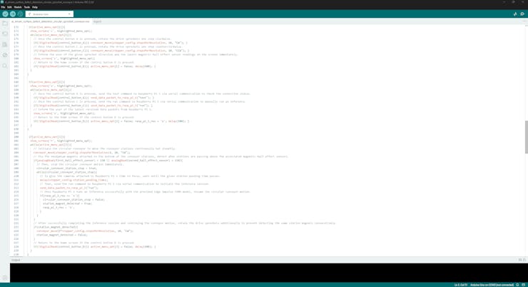
Circular Conveyor - Step 5: Designing the circular conveyor controller PCB (4-layer) as a Raspberry Pi 5 shield (hat)

After programming the ATmega328P and ensuring all electronic components performed features as expected, I started to work on designing the circular conveyor controller PCB layout. After developing distinct PCBs for my proof-of-concept projects, I came to the conclusion that designing PCB outlines and structures (silkscreen, copper layers, etc.) directly on Autodesk Fusion 360 works best for my development process. Creating PCB digital twins allows me to simulate complex 3D mechanical systems compatible with the PCB part placement and outline before sending my PCB designs for manufacturing. In this case, designing the layout on Fusion 360 was a necessity rather than a choice since I wanted to design the conveyor controller PCB as a unique Raspberry Pi 5 shield (hat), reducing the board footprint as much as possible.

As I was working on the conveyor PCB layout, I leveraged the open-source CAD file of Raspberry Pi 5 to obtain accurate measurements:

✒️ Raspberry Pi 5 (Step) | Inspect

#️⃣ First, I drew the PCB outline to make sure I left enough clearance for connecting the FPC camera connection cables to the dual-CSI ports.

#️⃣ Then, I added a circular opening (hole) for a cooling fan (40 mm x 40 mm) and ensured that the outline had enough clearance to attach its cable to the Pi 5 fan header.

❗ While conducting my experiments, I noticed that my Raspberry Pi 5's temperature increased to the point of a potential bottleneck, especially in the case of processing real-time image buffers produced by two different camera modules (regular Wide and NoIR Wide) simultaneously. Thus, to design a feature-rich shield (hat), I decided to add a built-in cooling fan on the top of the PCB, supporting the heatsinks affixed to the Raspberry Pi 5.

#️⃣ Finally, I thoroughly measured the areas of the electrical components with my caliper and placed them in the borders of the PCB outline diligently, including the 40-pin female pin header, which would be on the back of the PCB for attaching the shield onto the Raspberry Pi 5.

#️⃣ In the spirit of designing an authentic shield, I wanted to add Pikachu as a part of the PCB outline, emphasizing the power connectors :)

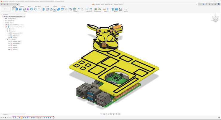
After designing the PCB outline and structure, I imported my outline graphic to KiCad 9.0 in the DXF format and created the necessary circuit connections to complete the circular conveyor PCB layout.

As I had already tested all electrical components on the breadboard, I was able to create the circuit schematic effortlessly in KiCad by following the prototype connections.

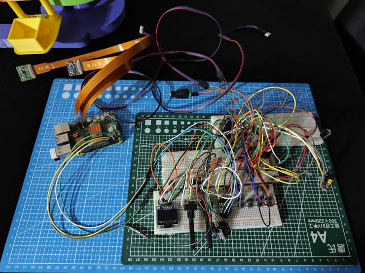
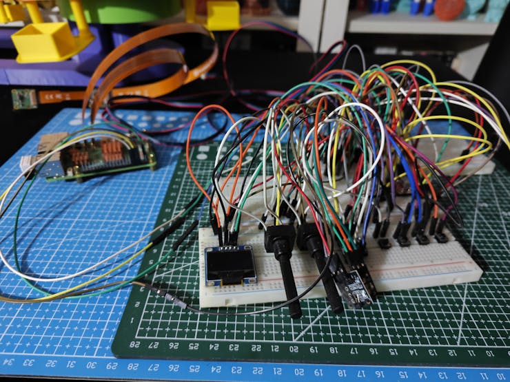
Before drawing connection lines to design the overall PCB layout, I noticed that a 2-layer PCB layout would be too restrictive for my compact part placement and unique PCB shape. In this regard, I decided to design a 4-layer PCB layout, which allowed me to create ground and power-oriented planes.

#️⃣ To increase the layer number on the KiCad PCB Editor, I navigated to File ➡ Board Setup ➡ Board Stackup ➡ Physical Stackup and selected the number of copper layers as 4.

After configuring the 4-layer PCB layout settings, I completed the circular conveyor controller PCB layout design layer-by-layer.

 

 

 

Circular Conveyor - Step 5.1: Soldering and assembling the circular conveyor controller PCB

After completing the circular conveyor controller PCB layout, I utilized ELECROW's high-quality regular PCB manufacturing service to fabricate my PCB design. For further inspection, I provided the fabrication files on the project GitHub repository. To replicate this device, you can order this PCB directly from my ELECROW community page.

#️⃣ After receiving my PCBs, I soldered electronic components and pin headers via my TS100 soldering iron to place all parts according to my PCB layout.

📌 Component assignments on the circular conveyor controller PCB:

U1 (ATmega328P-PU)

Y1 (16.000 MHz Crystal)

C1, C2 (22 pF Ceramic Capacitor)

C3 (100nF Ceramic Capacitor)

C4 (10uF 250V Electrolytic Capacitor)

R1 (10K Resistor)

DR1, DR2 (Headers for A4988 Stepper Motor Driver)

Motor1, Motor2 (Headers for Nema 17 [17HS3401] Stepper Motor)

Mg1, Mg2, (Headers for Magnetic Hall-effect Sensor Module [KY-003])

RV1, RV2 (Long-shaft Potentiometer [B4K7])

B1 (Headers for Logic Level Converter)

C_B1, C_B2, C_B3, C_B4, Reset1 (6x6 Pushbutton)

SSD1306 (Headers for SSD1306 OLED Display)

FT232RL1 (Headers for FTDI Adapter)

J1 (40-pin Female Header for Raspberry Pi 5)

J_5V_1, J_12V_1 (DC Barrel Female Power Jack)

J_5V_2, J_12V_2 (Headers for Power Supply)

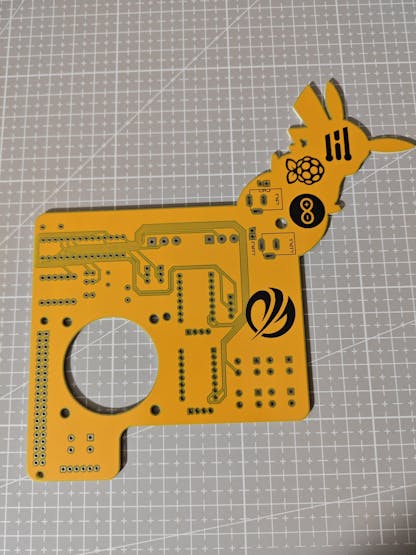
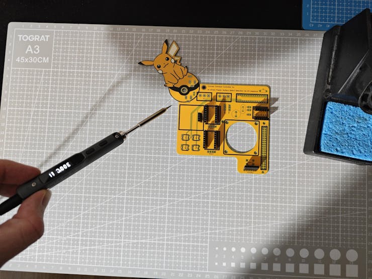
#️⃣ I soldered the 40-pin female header (20x2) to the back of the conveyor controller PCB since I designed the PCB as a Raspberry Pi 5 shield (hat).

#️⃣ After completing soldering components, I connected the cooling fan to the top of the PCB via its integrated M3 screw-nut pairs.

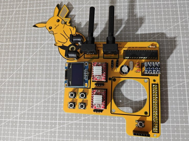
#️⃣ Then, I attached the remaining sensors and modules via their associated headers. I also affixed knobs to the long-shaft potentiometers to provide a more intuitive controller interface.

#️⃣ Even though I did not add a dedicated USB port to the PCB to minimize the shield footprint as much as possible, it is still possible to upload code files to the onboard ATmega328P chip by attaching the FTDI adapter to the PCB.

#️⃣ After ensuring the conveyor controller PCB operated as intended, I fastened it onto the Raspberry Pi 5 via the 40-pin header. Then, I attached the cooling fan cable to the Pi 5's dedicated fan header.

❗ DISCLAIMER: As I was developing the controller PCB, I utilized a white SSD1306 display directly attachable to the dedicated screen header. Nonetheless, while designing mechanical components, I decided to use a blue-yellow SSD1306 display instead of the white display version. Since the blue-yellow version has VCC and GND pins swapped, it must not be connected to the dedicated header directly. Hence, I connected the blue-yellow SSD1306 display via jumper wires to the PCB.

❗ If you want to replicate this project and PCB, a directly connectable SSD1306 display must have this pinout: VCC - GND - SCL - SDA

 

 

 

Circular Conveyor - Step 6: Developing custom mechanical components and parts to build a full-fledged circular sprocket-chain conveyor mechanism utilizing Hall-effect sensors for accurate positioning

In the spirit of developing a proof-of-concept research project, I wanted to showcase my concept of detecting plastic surface anomalies via the direct application of UV (ultraviolet) radiation in an industrial-grade setting. Therefore, I designed this circular sprocket-chain conveyor from the ground up, including custom ball bearings and multi-part chain.

Developing the complex mechanical parts of this circular conveyor was a strenuous process since I needed to go through five different iterations, not counting minor clearance corrections. After my adjustments, every feature of the final version of the automation mechanism worked as planned and anticipated, except that the stepper motors (Nema 17) around which I designed the primary internal gears could not handle the extra torque applied to my custom-designed ball bearings (with 5 mm steel beads) after I recalibrated the chain tension with additional tension pins, leading me to record some features by removing or loosing the chain for the demonstration videos.

I heavily modified my previous data collection rig to design the dual camera stands, elongated camera lens mounts, UV light source mounts, and the plastic object carriers.

As I was working on the circular conveyor mechanism, I leveraged some open-source CAD files to obtain accurate measurements:

✒️ Nema 17 (17HS3401) Stepper Motor (Step) | Inspect

✒️ Raspberry Pi Camera Module v3 (Step) | Inspect

✒️ Raspberry Pi 5 (Step) | Inspect

The pictures below show the final version of the circular conveyor mechanism on Fusion 360. I will explain all of my design choices and assembly process thoroughly in the following steps.

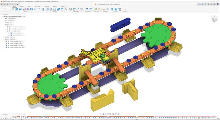
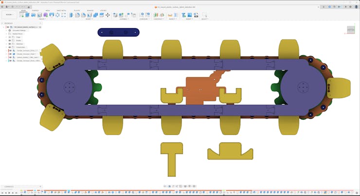
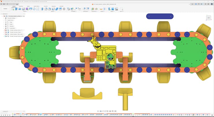
As a frame of reference for those who aim to develop a similar research project, I shared the design files (STL) of each mechanical component of this circular conveyor as open-source on the project GitHub repository.

🎨 As mentioned earlier, I sliced all the exported STL files in Bambu Studio and printed them using my Bambu Lab A1 Combo. In accordance with my color theme, I utilized these PLA filaments while printing 3D parts of the circular conveyor:

• PLA+ Peak Green
• PLA+ Very Peri
• Hyper Speed Orange
• Hyper Speed Yellow
• Hyper Speed Blue

The pictures below demonstrate the overview of the individual 3D parts of the earliest version of the circular conveyor mechanism during my initial ball bearing clearance review process. In later development stages, while going through different iterations, I modified some component designs and added chain tensioning parts as explained in the following steps.

 

 

 

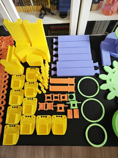
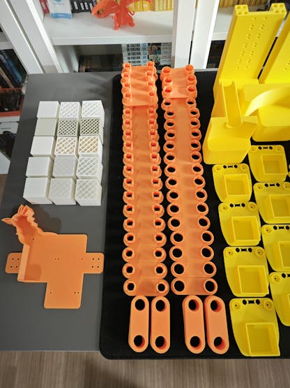
Circular Conveyor - Step 6.a: Designing the circular conveyor sprocket driver mechanism with a custom internal gear and ball bearing

#️⃣ First, I calculated the inner and outer gear radii of the internal gear mechanism.

#️⃣ The inner circle and the outer circle must be tangent circles, intersecting at a single point.

#️⃣ Then, I utilized the built-in SpurGear script to generate gears based on the inner and outer circles.

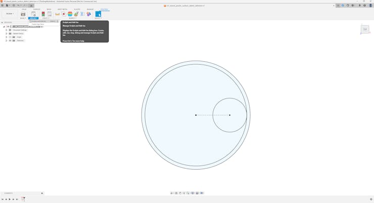
#️⃣ By modifying the inner gear, I created the primary driver gear attachable to the shaft of the Nema 17 stepper motor.

#️⃣ Around the Nema 17 stepper motor, I designed the base of the conveyor chain driver.

#️⃣ To make the driver base easily modifiable, I designed the base shaft carrying the custom ball bearing as a separate component.

#️⃣ Based on 5 mm steel balls (beads), I designed the custom ball bearing in three parts, making adjusting bearing pressure and stress effortless.

• Inner ring
• Outer ring [Top]
• Outer ring [Bottom]

#️⃣ By modifying the outer gear of the internal gear mechanism, I created the outer gear of the conveyor driver, pivoted by the custom ball bearing.

#️⃣ Finally, by using the SpurGear script, I designed the sprocket that moves the conveyor chain. As I was going through different design iterations, I heavily modified the usual spur gear layout to get the optimal results while moving the conveyor chain.

#️⃣ As discussed, I developed the circular conveyor mechanism to drive the conveyor chain via two drivers simultaneously to create a stable system. Thus, I mirrored the first conveyor driver to create the second conveyor driver.

#️⃣ Nonetheless, due to the produced angular momentum, it would not be wise to attach the conveyor chain to separated and unsupported drivers. In this regard, I designed the driver guide rails with triangular mortise and tenon joints.

 

 

 

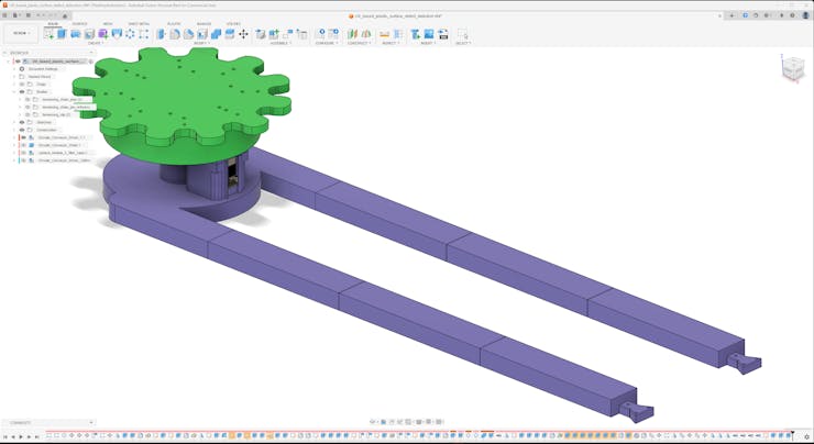
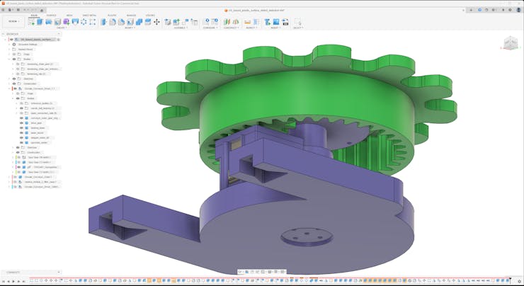
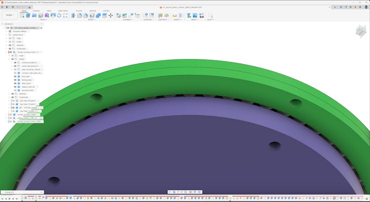
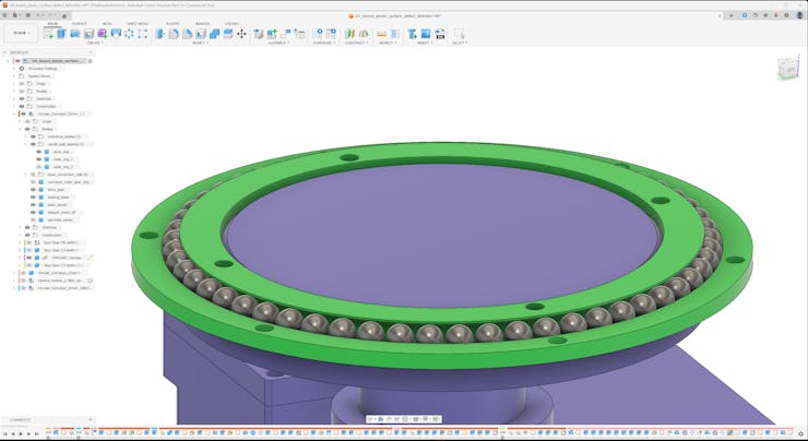
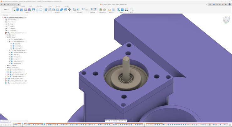
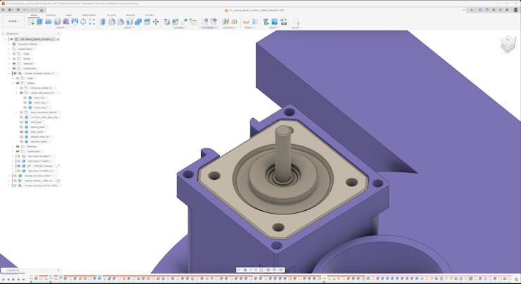
Circular Conveyor - Step 6.a.1: Printing and assembling the circular conveyor sprocket driver mechanism

#️⃣ First, on Autodesk Fusion 360, I exported all conveyor driver components as individual STL files.

#️⃣ Then, I sliced the exported parts in Bambu Studio, providing an intuitive user interface for adjusting slicer settings even for complex structures.

#️⃣ Since the driver base shaft carries the custom ball bearing, pivoting the sprocket, I utilized the built-in height range modifiers to increase the wall loop (perimeter) number of potential weak points to 3.

#️⃣ I also increased the wall loop (perimeter) number to 3 for the custom bearing parts and the primary driver (inner) gear.

#️⃣ For the remaining components, I selected the sparse infill density as 10% instead of 15%.

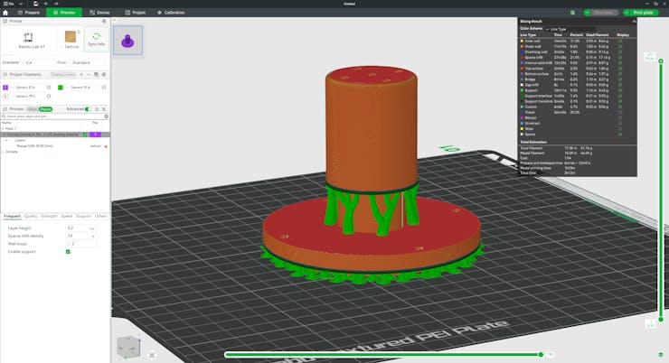
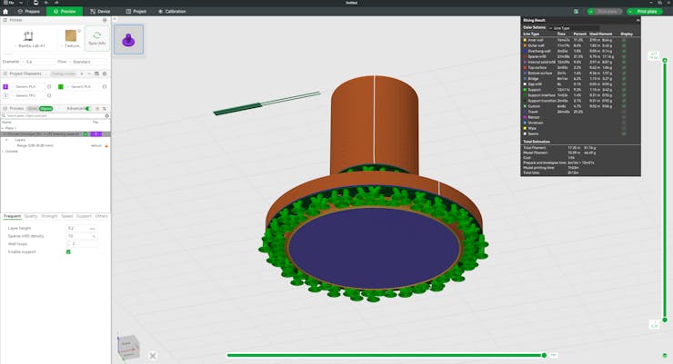
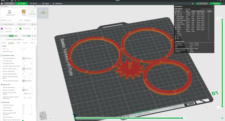
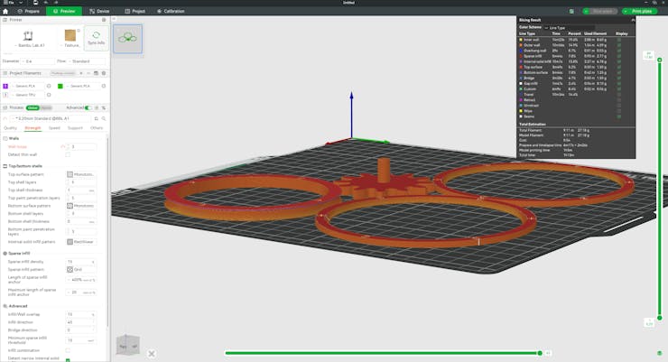
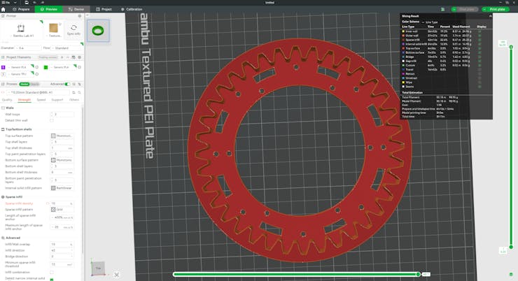
#️⃣ Since threaded inserts use heat to bond by melting the plastic, they reinforce M3 screw connections more than any other method. Hence, I utilized my TS100 soldering iron with its special heat set tip kit to install M3 brass threaded inserts to the conveyor driver base shaft to strengthen its connection with the driver base and the custom ball bearing.

#️⃣ Then, I assembled the custom ball bearing by utilizing 5 mm steel balls (beads), M3 washers, screws, and nuts. I chose not to permanently fasten the outer rings of the ball bearing since I wanted to adjust the bearing stress while building the conveyor mechanism.

#️⃣ I placed the Nema 17 stepper motor into its slot and installed M3 inserts to attach the stepper motor lid to the driver base via M3 threaded bolts.

#️⃣ Then, I fastened the primary driver gear (inner) to the stepper motor shaft.

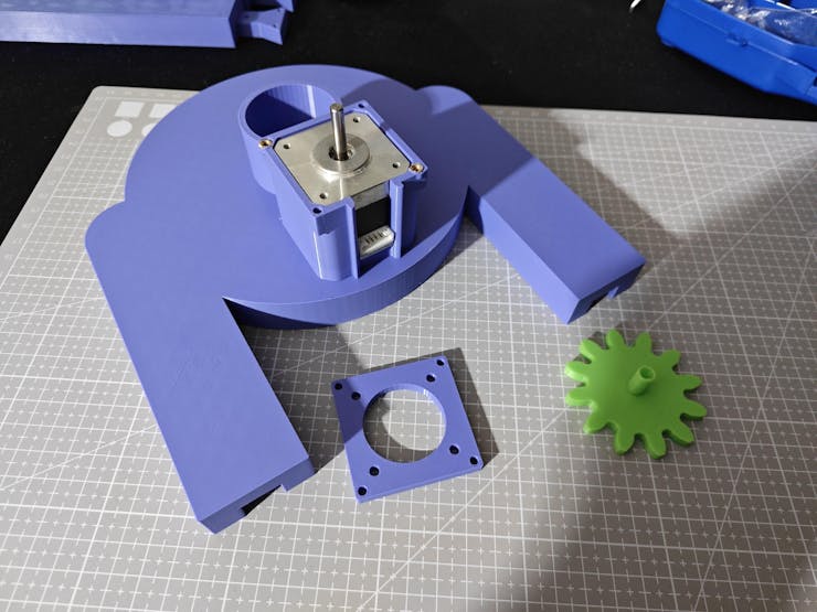
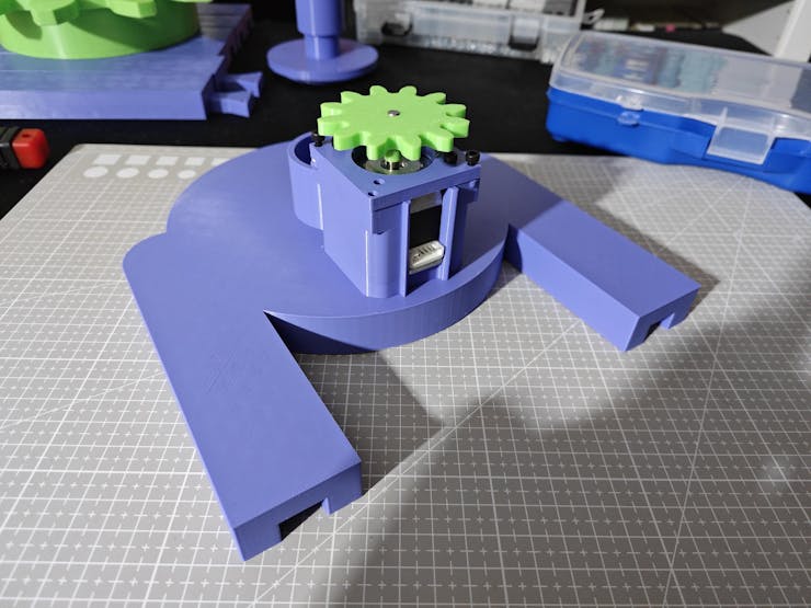
#️⃣ After affixing the conveyor driver base shaft to the driver base via M3 screws successfully, I attached the custom ball bearing to the top of the base shaft via M3 screws through the installed M3 inserts.

#️⃣ After installing M3 inserts to the outer gear of the conveyor driver for strengthening the sprocket connections (if necessary), moving the conveyor chain, I attached the outer gear to the custom ball bearing by employing the M3 screws already tensioning the outer rings of the bearing. While attaching the outer gear, I changed the tensioning M3 screws with longer ones to gain more clearance and added M3 washers between the ball bearing and the driver outer gear to reduce friction.

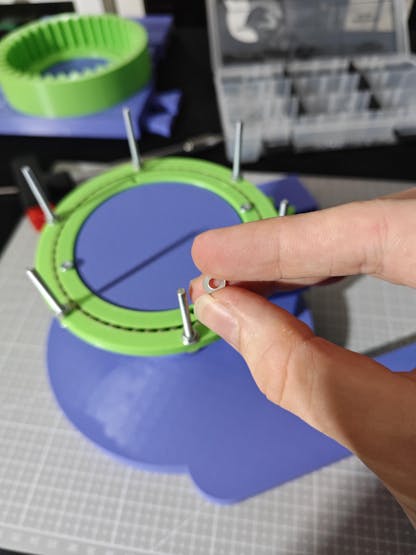
#️⃣ After completing the assembly of the first conveyor driver successfully, I assembled the second conveyor driver by following the exact same steps above.

 

 

 

 

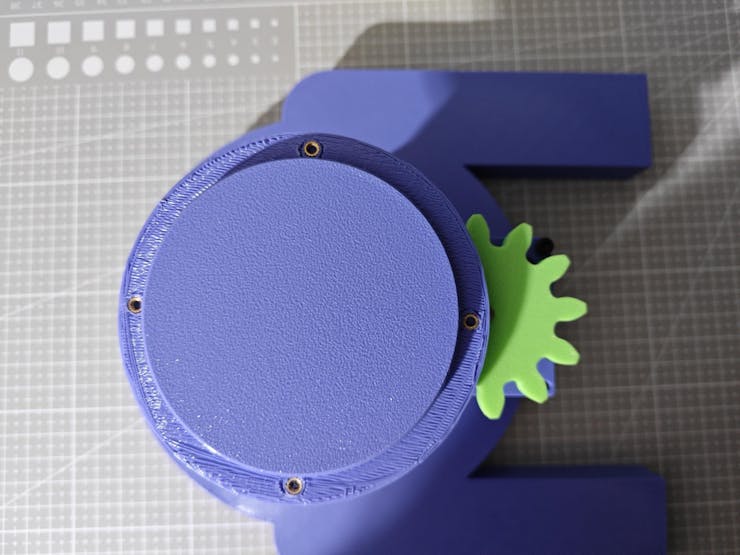
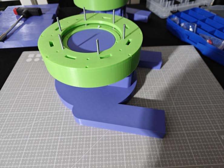
Circular Conveyor - Step 6.b: Designing the circular conveyor controller PCB mount and camera module 3 stations (regular Wide and NoIR Wide) based on the previous data collection rig

#️⃣ As mentioned earlier, I designed the dual camera stands, UV light source holders, and the camera lens mounts by heavily modifying my previous data collection rig.

#️⃣ First, I divided the rig bases to create separate UV strip and flashlight-compatible holders, letting me change UV light sources without disturbing the camera module cases or the plastic object carriers.

#️⃣ I utilized the same camera case and filter lens designs for the color gel and the UV bandpass filters. Nevertheless, I elongated the camera case mount to ensure the focal points of the camera modules (regular Wide and NoIR Wide) aligned with the center of the plastic object surfaces, carried by the plastic object carriers.

#️⃣ Based on the conveyor controller PCB outline, I designed an authentic PCB case bridging two camera stand racks while encapsulating the Raspberry Pi 5.

 

 

 

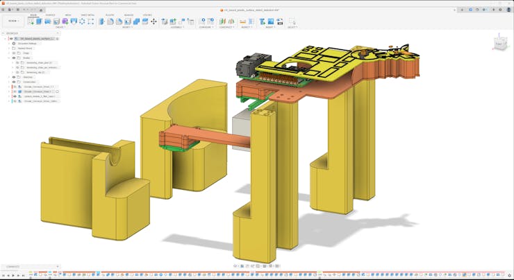
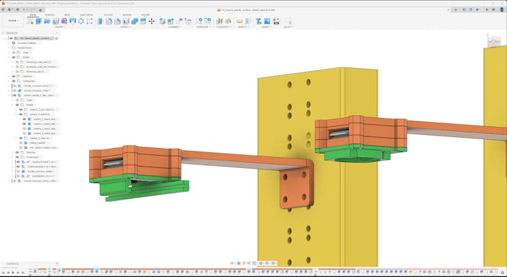
Circular Conveyor - Step 6.b.1: Printing and assembling the circular conveyor PCB mount and camera stations

#️⃣ While slicing the UV light source holders and the camera stands, I selected the sparse infill density as 5% and applied the gyroid sparse infill pattern to print lightweight components as strong as possible.

#️⃣ For the remaining parts, I used the usual slicer settings.

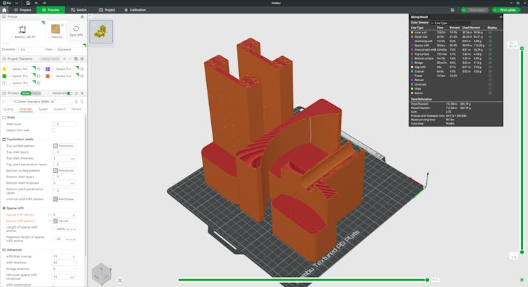
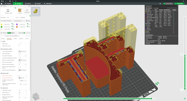
#️⃣ To reinforce the connection between the PCB case and the camera stand racks, I installed M3 inserts and employed M3 threaded bolts.

#️⃣ Then, I attached the dedicated Hall-effect sensor mounts directly to the camera stand racks via M3 screws.

 

 

 

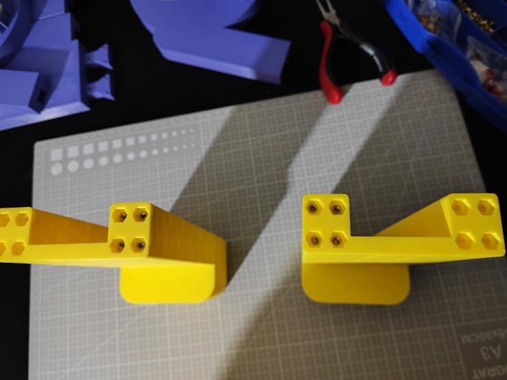
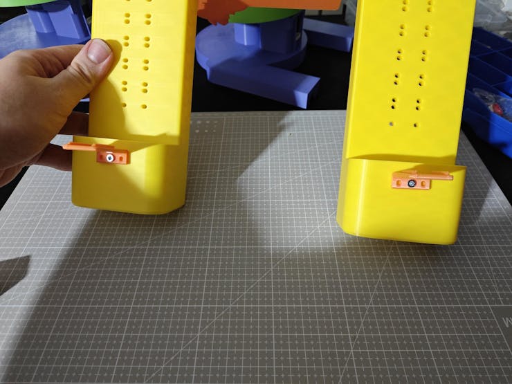
Circular Conveyor - Step 6.c: Affixing sprockets to the conveyor drivers and attaching the guide rails

#️⃣ Similar to the camera stands, I selected the sparse infill density as 5% while applying the gyroid sparse infill pattern to make the guide rails lightweight but robust.

#️⃣ First, I attached the sprockets to the outer gears of the conveyor drivers via the pre-installed M3 screws, already tensioning the outer gears and the outer rings of the custom ball bearings.

❗ The pictures below demonstrate the very first iteration of the sprockets. While developing the conveyor mechanism, I heavily modified the sprocket design to move the conveyor chain most efficiently.

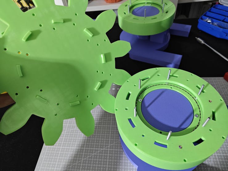
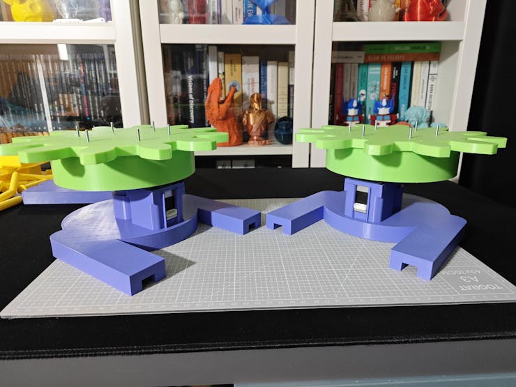
#️⃣ Then, I connected the two separate conveyor driver bases via the guide rails. Although I added holes to tighten the rail connections via M3 screws, the integrated triangular mortise and tenon joints were more than enough to move the conveyor chain stably.

 

 

 

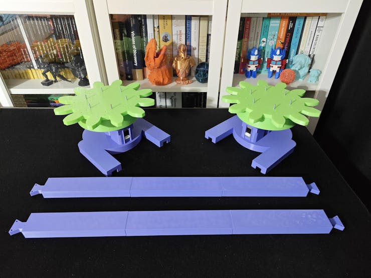
Circular Conveyor - Step 6.d: Designing the chain outer and inner plates with annular snap fit joints (roller-pin connection)

#️⃣ Since I wanted to design a unique multi-part conveyor chain instead of purchasing a commercial conveyor chain, I scrutinized various production line system documentation to decide the best chain type for my use case.

#️⃣ After my research, I decided to design my chain composed of these interlocking parts:

• Outer plate
• Outer plate with pins
• Inner plate
• Inner plate with roller

#️⃣ I designed the outer plate pins as annular snap fit joints, which are suitable for high-stress applications and distribute stress uniformly. In this regard, it is possible to assemble or disassemble the chain at any length without additional tools or parts.

#️⃣ Based on the length of one chain link, I calculated the required chain links covering the driver sprockets and the distance between them.

 

 

 

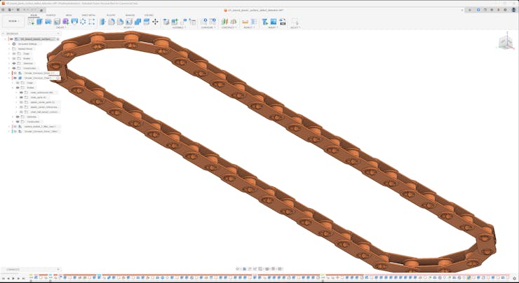
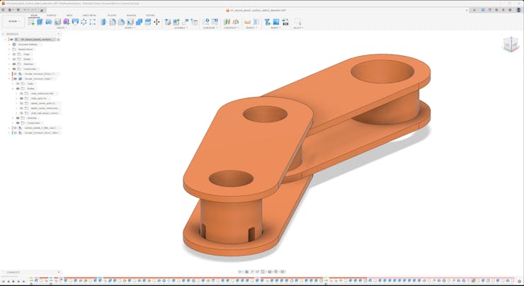
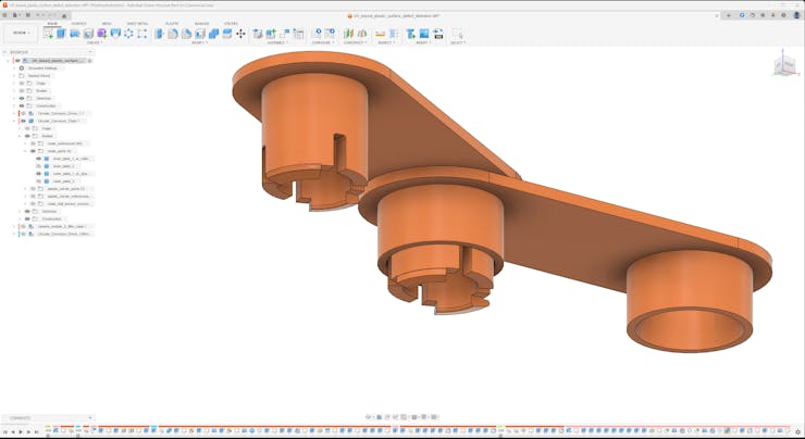
Circular Conveyor - Step 6.d.1: Designing custom plastic object carriers compatible with neodymium magnets and aligning Hall-effect sensor mounts

#️⃣ After estimating the chain length and simulating the fully wrapped chain on Fusion 360, I was able to design the plastic object carrier structure precisely.

#️⃣ Since I had already aligned the focal points of the camera modules and the center of the target plastic object surfaces, I derived the base of the plastic object carrier by directly encasing the target objects.

#️⃣ By knowing the distance between the bottom of the plastic object carrier and the top of the conveyor chain, I designed two separate pins to attach the object carrier to an outer chain link.

#️⃣ To the back of the carrier base, I added slots for one circular neodymium magnet (8 mm) and two rectangular neodymium magnets (10 mm x 5 mm). Since I did not want to use fasteners, I specifically designed snap fit slots for the magnets, applying the strain produced by the expanded plastic.

#️⃣ To design an accurate Hall-effect sensor mount attachable to the camera stands, I took the precise measurements of the module via my caliper. Then, I made sure the center of the Hall-effect sensor (placed at the front of the module) aligned with the center of the circular neodymium magnet under the plastic object carrier, leading to optimal sensor readings while moving the conveyor chain.

#️⃣ After successfully designing the first plastic object carrier based on the target object, I copied a plastic carrier to each second outer chain link to simulate the final state of the conveyor chain.

 

 

 

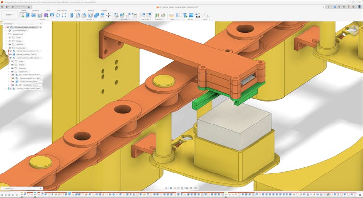
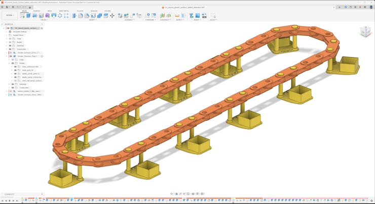
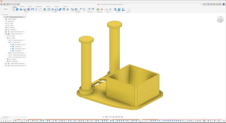
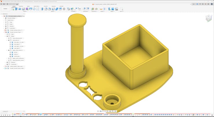
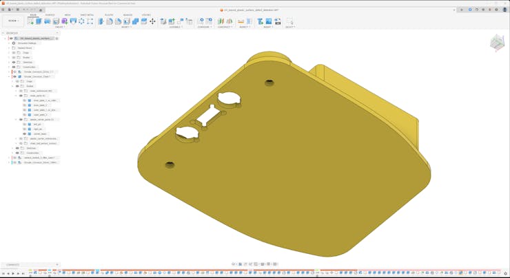
Circular Conveyor - Step 6.d.2: Printing and assembling the conveyor chain links and plastic carriers

#️⃣ Since the outer plate pins carry the most load and need to distribute stress while moving the conveyor chain, I decided to boost outer plate strength by basically printing their pins as solid plastic. In this regard, I increased the wall loop (perimeter) number to 4 while slicing them on Bambu Studio.

#️⃣ For the remaining chain parts, I utilized the usual slicer settings.

#️⃣ To reduce the total chain weight while preserving its rigidity, I also sliced all plastic object carrier components with the usual settings.

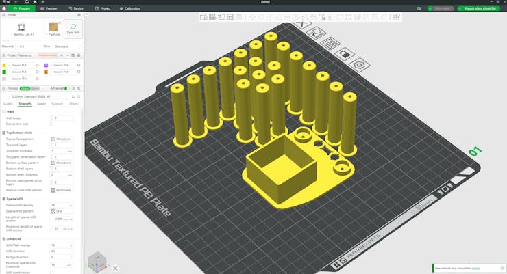
#️⃣ I started to assemble the conveyor chain with two inner chain links and one outer chain link.

#️⃣ After testing the flexibility of the first connected chain links, I proceeded to complete the assembly of the whole conveyor chain.

#️⃣ Then, I attached neodymium magnets to each plastic object carrier base via their dedicated snap fit slots.

• 1 x Circular neodymium magnet [8 mm]
• 2 x Rectangular neodymium magnets [10 mm x 5 mm]

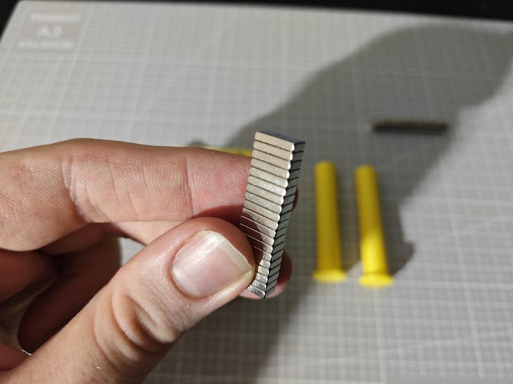
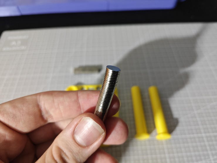
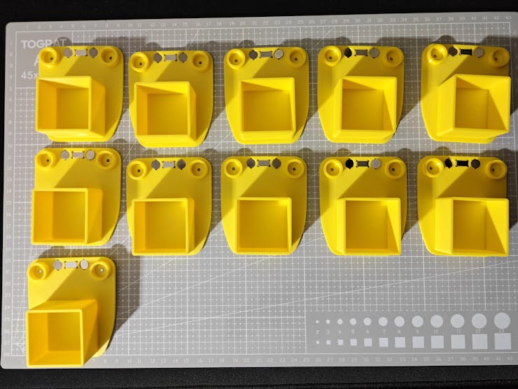
#️⃣ Finally, I connected plastic object carrier bases to each second outer chain link via the carrier pins by using M3 screws.

 

 

 

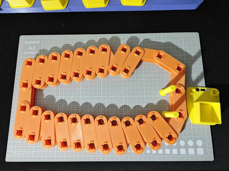
Circular Conveyor - Step 6.f: Overhauling my component design mistakes and recalibrating the chain tension by adding tension pins and a tensioning clip to fix chain sag

As discussed earlier, I needed to go through different iterations to overhaul some of my design mistakes. I omitted explaining the minor iterations due to clearance issues, as they did not impact the final version of the conveyor mechanism. Nevertheless, I needed to heavily modify some mechanical components and change the final mechanism to incorporate the major design iterations outlined below.

All of the major issues stemmed from my faulty simulations of mechanical component attributes and interactions.

#️⃣ First, there was too much friction between the chain links and the sprockets due to the length of the gear teeth, even though I assessed that the sprockets should have moved the conveyor chain perfectly on Fusion 360. Nonetheless, the friction issues were probable since even the quality of the sprocket surface finish could cause extra friction or clearance problems.

#️⃣ In this regard, I reiterated the sprocket design until achieving the optimal results while moving the conveyor chain.

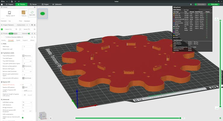
#️⃣ After solving the friction issues, the conveyor chain was moving smoothly. However, there was an even bigger problem: the sag of the conveyor chain was more than I calculated, rendering the neodymium magnets under the plastic object carrier bases not aligned with the Hall-effect sensor modules.

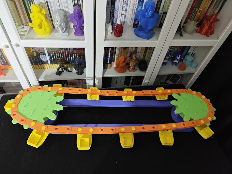
#️⃣ After studying my previous simulations, I concluded that I had missed the weight of the additional perimeters of the outer plates and the tilt of my floor while estimating the chain sag.

#️⃣ Therefore, I needed to recalibrate the chain tension to ensure the carriers were aligning with the magnetic sensors. After mulling over countless solutions, I decided to add tensioning pins to the conveyor chain.

#️⃣ Since I added tensioning pins to each second outer chain link, I was able to disassemble the conveyor chain at different points to estimate the required force to tension the chain enough for realignment. Basically, I utilized a twine to reconnect the separated chain links and counted how many times I wrapped the twine until obtaining the required tension.

#️⃣ After estimating the required force, I realized that I could tension the conveyor chain by removing two inner chain links with one outer chain link and adding a tensioning clip instead.

#️⃣ Since each second outer chain link was connected to a plastic object carrier, I would have had to discard one object carrier while tensioning the conveyor chain via the tensioning clip. Therefore, I designed the tensioning clip to hold the discarded carrier at the same level as the outer chain links.

#️⃣ Of course, adding this much unprecedented tension to the conveyor chain rendered the Nema 17 stepper motors not able to handle the extra torque applied to my custom-designed ball bearings (with 5 mm steel beads). Thus, as mentioned earlier, I needed to record some features related to sprocket movements (affixed to outer gears pivoted on the ball bearings) by removing or loosening the chain for the demonstration videos.

 

 

 

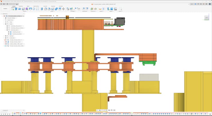
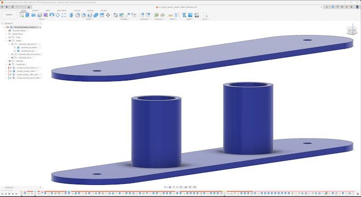
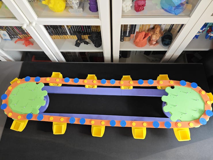
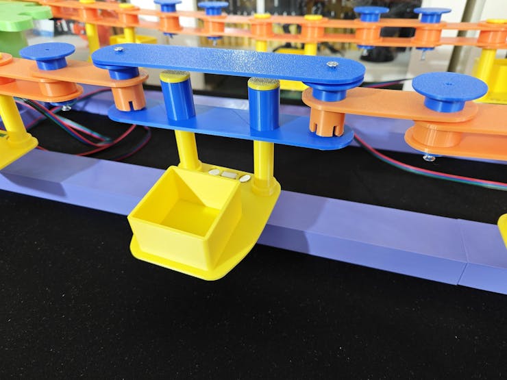
Circular Conveyor - Step 6.g: Assembling unique camera filter lenses and attaching the Raspberry Pi 5 with the circular conveyor controller PCB (shield) to the camera stations

#️⃣ Due to the elongated camera case mount, I needed to strengthen the camera module case parts to ensure the camera modules would not shake while moving the plastic object carriers. Thus, I increased the wall loop (perimeter) number to 4 while slicing them on Bambu Studio.

#️⃣ For the same reason, I also sliced the Hall-effect sensor module mounts with extra perimeters.

#️⃣ The assembly of the multi-part camera module cases was the same as the camera case of the data collection rig because I only modified the length of the camera case mount.

#️⃣ Even though I printed new camera case parts with increased perimeters, I decided to utilize the previously printed camera filter lenses, as I had already permanently affixed the glass UV bandpass filter to its dedicated camera lens.

 

 

 

 

 

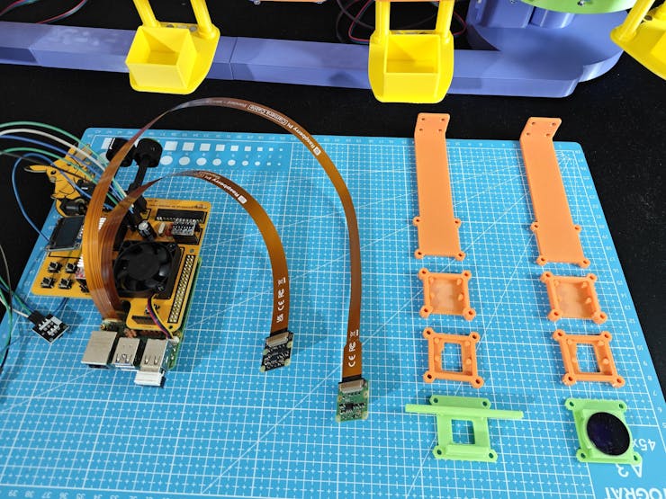
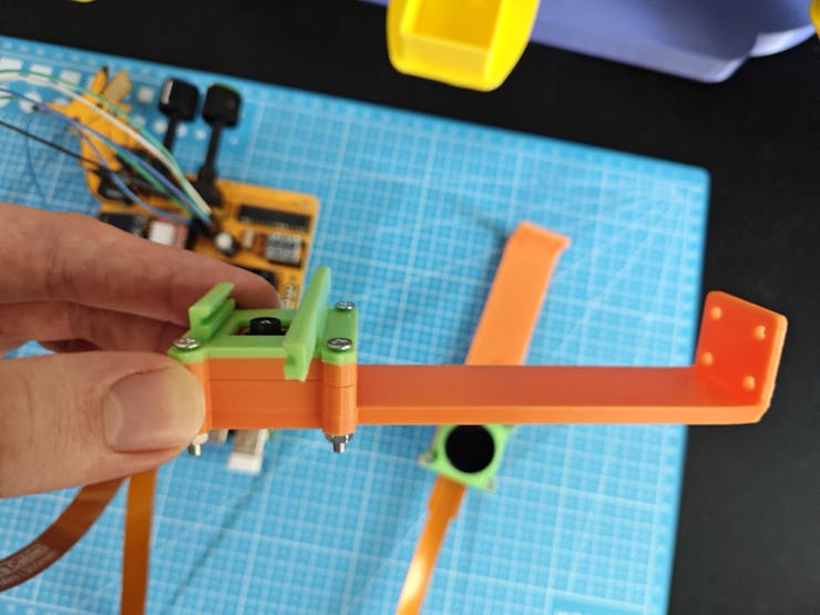
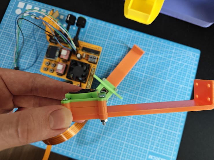
#️⃣ After assembling the camera module cases of regular Wide and NoIR Wide camera modules, I fastened the Raspberry Pi 5 to the PCB case via M2 screws, nuts, and washers. To raise the Raspberry Pi 5 from the PCB case surface, I utilized extra M2 nuts.

#️⃣ Then, I attached camera module case mounts to the racks of the camera stands via eight M3 screw-nut pairs. Although separated, the camera stand racks are the same as those of the previous data collection rig bases, leading to persistent results while collecting new UV-applied plastic surface images.

#️⃣ After connecting the power supply to the Raspberry Pi 5, I attached the conveyor controller PCB to the Raspberry Pi 5 via its 40-pin female header. Since I specifically designed the PCB case edges to support the heavy side of the conveyor PCB to reduce the load on the pin header, I did not encounter any connection problems.

 

 

 

 

 

 

 

#️⃣ Finally, I fastened the Hall-effect sensor modules to their dedicated mounts on the camera stands via a hot glue gun.

 

#️⃣ After making sure the FPC camera connection cables were firmly attached to the camera cases using zip ties, I concluded the PCB case assembly.

 

 

 

 

 

 

 

 

 

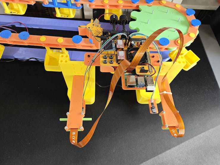
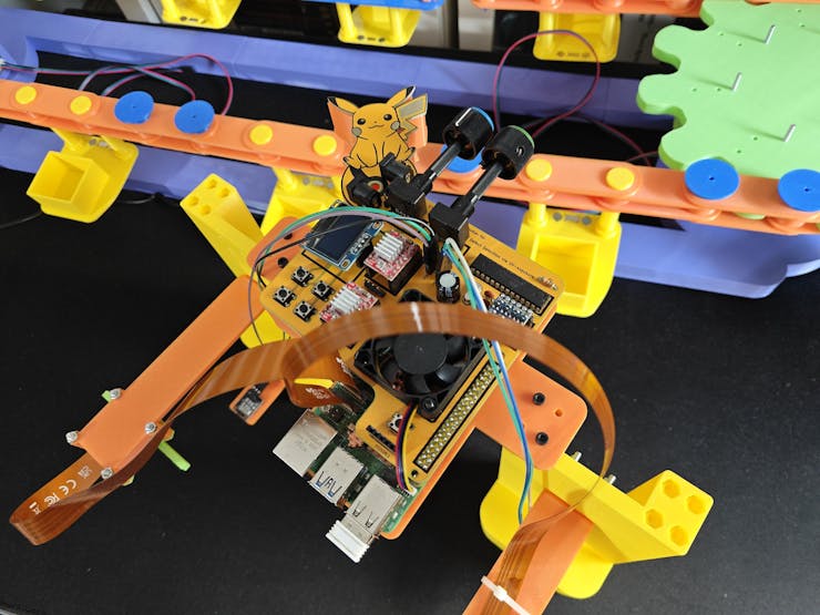
Circular Conveyor - Step 6.h: Positioning Hall-effect sensors, plastic objects, and UV light sources

❗ As I was completing the assembly of the final version of the circular conveyor mechanism, I decided to switch the white SSD1306 display for the blue-yellow SSD1306 display. As mentioned earlier, I needed to connect the blue-yellow version via jumper wires since it has VCC and GND pins swapped. Therefore, I decided to fasten the blue-yellow SSD1306 screen to the front of the first camera stand rack via the hot glue gun.

⚙️ Positioning the camera stand racks bridged by the conveyor controller PCB case between the guide rails and aligning the Hall-effect sensors with the neodymium magnets:

 

 

 

 

 

⚙️ Installing UV light sources into their respective holders in the flashlight format and the strip format:

 

 

 

 

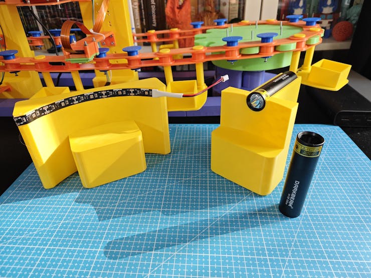
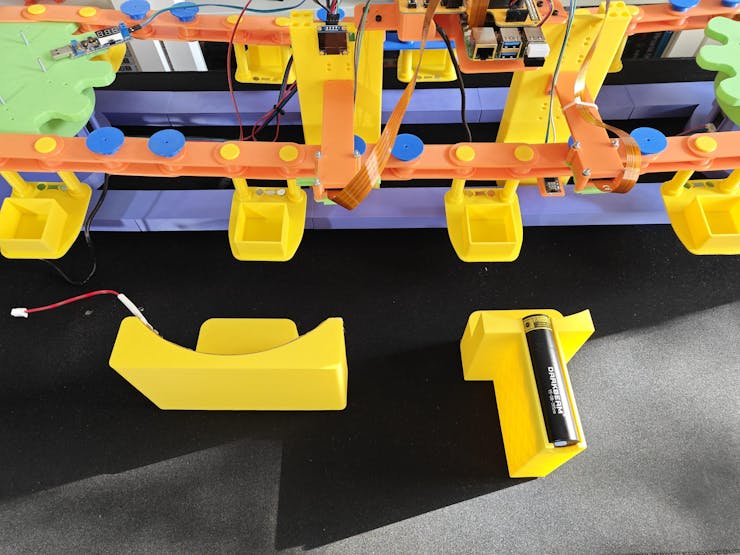
⚙️ Placing the color gel filters into the dedicated camera filter lens:

 

 

 

 

 

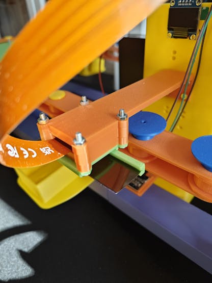
⚙️ Putting the plastic objects into their dedicated carriers connected to the conveyor chain:

 

 

 

 

 

 

 

 

 

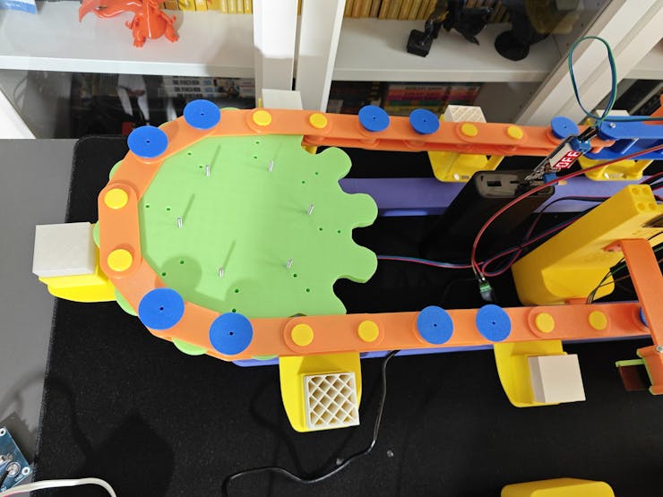
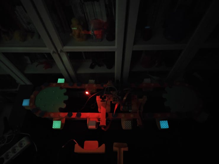
⚙️ Testing camera modules (regular Wide and NoIR Wide), UV light sources (275 nm, 365 nm, and 395 nm), and the Hall-effect sensors:

 

 

 

 

 

 

 

 

 

 

 

 

 

 

 

 

 

 

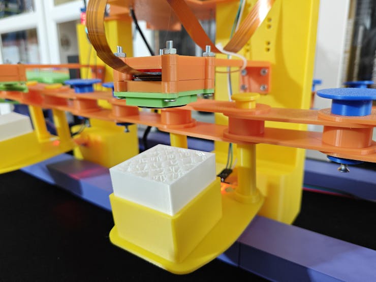
Circular Conveyor - Step 7: Creating an account to utilize Twilio's SMS API

Even before starting to develop the web dashboard of the circular conveyor, I knew that I wanted to enable the web dashboard to inform the user of the detected plastic surface anomalies via SMS. Thus, I decided to utilize Twilio's SMS API since Twilio provides a trial text messaging service to transfer an SMS from a virtual phone number to a verified phone number internationally. Furthermore, there are official Twilio helper libraries for different programming languages, including PHP, enforcing its suite of APIs.

#️⃣ First, to be able to access trial services, I navigated to the Account section and created a new account, which is a container for Twilio applications.

 

 

 

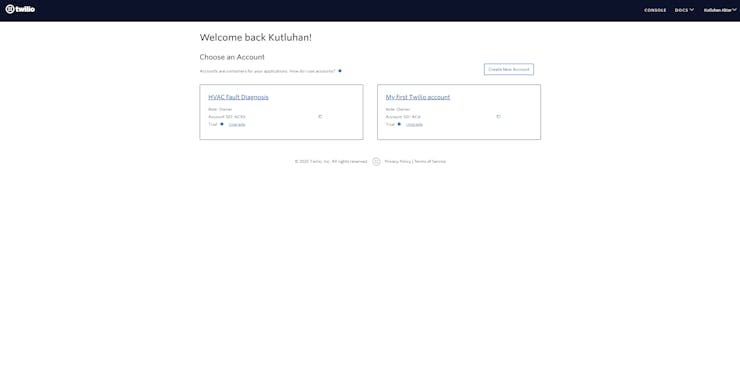
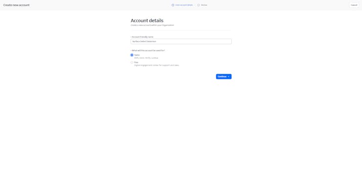
#️⃣ After verifying my phone number for the newly created account (container), I configured the initial account settings for implementing the Twilio SMS API in PHP.

 

 

 

 

 

#️⃣ To enable the SMS service, I navigated to Messaging ➡ Send an SMS and obtained a free 10DLC virtual phone number.

 

 

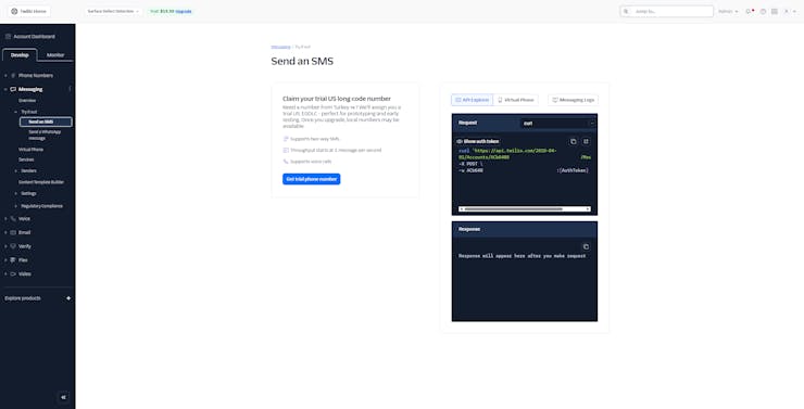
#️⃣ Then, I tested the trial SMS service by sending a message to my verified phone number via the Twilio web interface.

 

 

#️⃣ If the Twilio console throws a permission error, you might need to go to the Geo permissions section to add your country to the allowed recipients.

 

 

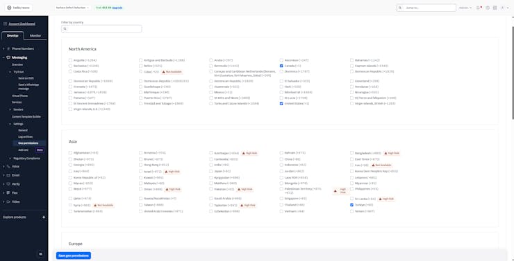
#️⃣ After adjusting allowed recipients, I was able to send the test message from the console without a problem.

 

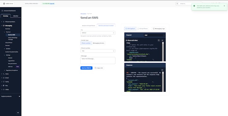
#️⃣ After making sure the Twilio SMS service worked as anticipated, I navigated to the Account Info section to obtain the required account credentials (SID and auth token).

#️⃣ Finally, I installed the Twilio PHP helper library to enable the web dashboard to access the SMS API locally for transferring notification messages.

 

 

 

 

Circular Conveyor - Step 8: Developing a feature-rich circular conveyor web dashboard to observe and sort the latest inference results on Raspberry Pi 5

As discussed earlier, I decided to develop a web dashboard for the circular conveyor mechanism to allow the user to observe the latest inference results in real-time and sort them by the camera module type — regular Wide or NoIR Wide, leading to pinpointing plastic surface anomalies by object more easily. As mentioned in the previous step, I also enabled the web dashboard to employ Twilio's SMS API to inform the user of the latest detected plastic surface anomalies. To ensure the web dashboard could access the latest inference results without any issues, I developed the web dashboard as I was setting up the FOMO-AD visual anomaly detection model on Raspberry Pi 5. I explained the web dashboard code files thoroughly in the following steps. Nonetheless, you can refer to the project GitHub repository if you want to download or inspect the code files directly.

The directory structure (alphabetically) of the circular conveyor web dashboard is as follows, under surface_defect_detection_dashboard as the application root folder:

• /anomaly_detection
• /fomo_ad_model
• ai-driven-plastic-surface-defect-detection-via-uv-exposure-linux-aarch64-v1.eim
• /inference_results
• uv_defect_detection_run_inference_w_rasp_5_camera_mod_wide_and_noir.py
• /assets
• /img
• /script
• dashboard_update.js
• index.js
• /style
• index.css
• root_variables.css
• /twilio-php-main
• anomaly_update.php
• class.php
• create_necessary_database_tables.sql
• database_secrets.php
• settings_update.php
• index.php

 

 

 

 

 

 

 

 

 

 

 

 

 

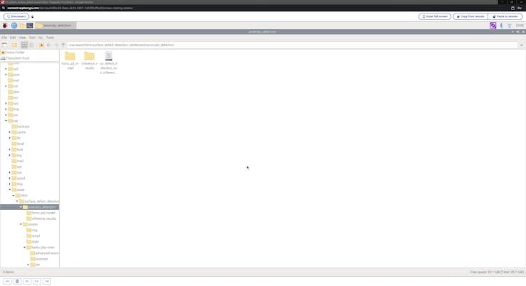
Circular Conveyor - Step 8.1: Constructing the necessary database tables on MariaDB

Since I had already set up the Apache server with the MariaDB database to develop the web dashboard on the Raspberry Pi 5, I was able to configure the required database settings on the terminal effortlessly.

#️⃣ First, I created a new MariaDB database named surface_detection by utilizing the integrated terminal prompt.

sudo mysql -uroot -p

create database surface_detection;

GRANT ALL PRIVILEGES ON surface_detection.* TO 'root'@'localhost' IDENTIFIED BY '';

FLUSH PRIVILEGES;

#️⃣ Then, by running these SQL commands on the terminal, I created two new database tables with the necessary data fields and inserted the initial dashboard states into the associated database table.

use surface_detection;

CREATE TABLE `notification_settings`(id int AUTO_INCREMENT PRIMARY KEY NOT NULL, cam_regular varchar(255), cam_noir varchar(255), sms_twilio varchar(255) );

INSERT INTO `notification_settings` (`cam_regular`, `cam_noir`, `sms_twilio`) VALUES ("activated", "activated", "activated");

CREATE TABLE `anomaly_results`( id int AUTO_INCREMENT PRIMARY KEY NOT NULL, cam_type varchar(255), detection varchar(255), img_file varchar(255), station_num varchar(255), detection_time varchar(255), server_time varchar(255) );

 

 

 

 

 

 

 

 

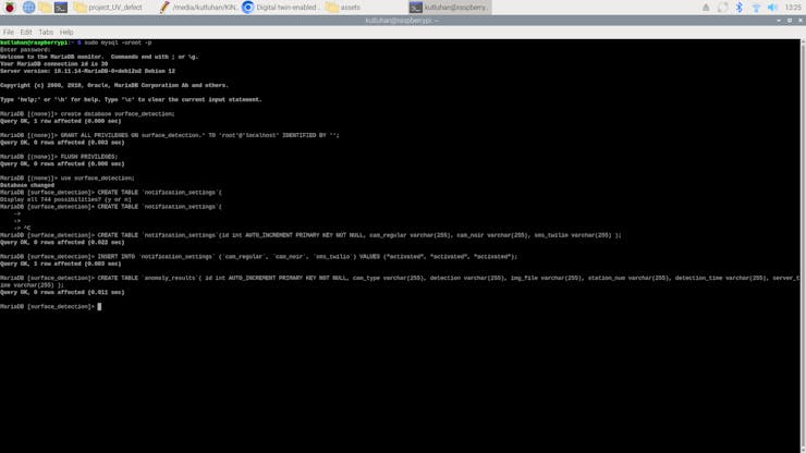
#️⃣ As mentioned, I developed the web dashboard and configured the FOMO-AD visual anomaly detection model simultaneously. In this regard, I needed to clear the inference results from the associated database table a few times during my experiments until the web dashboard was showing the inference results as intended. To achieve this, I dropped and recreated the associated database table by running these SQL commands.

DROP TABLE `anomaly_results`;

CREATE TABLE `anomaly_results`( id int AUTO_INCREMENT PRIMARY KEY NOT NULL, cam_type varchar(255), detection varchar(255), img_file varchar(255), station_num varchar(255), detection_time varchar(255), server_time varchar(255) );

 

 

 

 

Circular Conveyor - Step 8.2: Setting up the FOMO-AD (visual anomaly detection) model on Raspberry Pi 5

After installing my FOMO-AD visual anomaly detection model as an EIM binary for Linux (AARCH64) on the Raspberry Pi 5, I needed to configure some permission settings to integrate the FOMO-AD model into the web dashboard successfully.

#️⃣ Since the child directories and files under the root folder of the Apache server are restricted, I changed permissions to enable file creation and modification while running the web dashboard.

sudo chmod 777 /var/www/html

 

#️⃣ Since I copied the EIM binary — Linux (AARCH64) — after changing the root folder permissions, I changed the file permissions of the binary specifically to make it executable.

sudo chmod 777 /var/www/html/surface_defect_detection_dashboard/anomaly_detection/fomo_ad_model/ai-driven-plastic-surface-defect-detection-via-uv-exposure-linux-aarch64-v1.eim

 

 

 

 

Circular Conveyor - Step 8.3: Thorough file-by-file code documentation of the conveyor web dashboard

📁 create_necessary_database_tables.sql

⭐ Necessary SQL commands to create the required database tables with the initial states in the MariaDB database.

CREATE TABLE `notification_settings`(id int AUTO_INCREMENT PRIMARY KEY NOT NULL, cam_regular varchar(255), cam_noir varchar(255), sms_twilio varchar(255) );

INSERT INTO `notification_settings` (`cam_regular`, `cam_noir`, `sms_twilio`) VALUES ("activated", "activated", "activated");

CREATE TABLE `anomaly_results`( id int AUTO_INCREMENT PRIMARY KEY NOT NULL, cam_type varchar(255), detection varchar(255), img_file varchar(255), station_num varchar(255), detection_time varchar(255), server_time varchar(255) );

DROP TABLE `anomaly_results`;

 

📁 database_secrets.php

⭐ Enable the PHP-based MariaDB database connection via the integrated MySQLi extension.

// Database info.
$server = array(
	"server" => "localhost",
	"username" => "root",
	"password" => "",
	"database_name" => "surface_detection"
);

// Database connection credentials.
$_db_conn = mysqli_connect($server["server"], $server["username"], $server["password"], $server["database_name"]);

 

📁 class.php

#️⃣ To bundle all the functions to write a more concise script, I used a PHP class.

⭐ Import the required MariaDB database connection settings.

⭐ Include the Twilio PHP helper library and its required modules.

include_once "database_secrets.php";

// Include the Twilio PHP Helper Library. 
require_once 'twilio-php-main/src/Twilio/autoload.php';
use Twilio\Rest\Client;

⭐ Declare the necessary Twilio account (container) and phone number (trial and registered) information.

private $twilio_info = array(
									"sid" => "<__SID__>",
									"token" => "<__TOKEN__>",
									"to_phone" => "+16__________",
									"from_phone" => "+16_________"
	                            );

⭐ In the __init__ function:

⭐ Integrate the previously declared MySQL object with the passed database credentials into this PHP class.

⭐ Declare a new Twilio client instance (object).

public function __init__($_db_conn){
		// Init the MySQL object with the passed database credentials.
		$this->db_conn = $_db_conn;
		// Declare a new Twilio client instance (object). 
		$this->twilio = new Client($this->twilio_info["sid"], $this->twilio_info["token"]);		
	}

⭐ In the send_sms function, transfer the given text message as an SMS to the registered phone number through the Twilio SMS API.

protected function send_sms($message){
		$message = $this->twilio->messages
								->create($this->twilio_info["to_phone"], // to
										array(
												"from" => $this->twilio_info["from_phone"],
												"body" => $message
											 )
										);
		echo "Sent SMS SID: ".$message->sid;
	}

⭐ In the obtain_not_settings function, obtain the latest dashboard status states from the associated MariaDB database table.

public function obtain_not_settings(){
		$sql = "SELECT * FROM `$this->not_set_table` WHERE `id` = 1";
		$result = mysqli_query($this->db_conn, $sql);
		$check = mysqli_num_rows($result);
		if($check > 0){
			// If found successfully, return the registered notification settings.
			if($row = mysqli_fetch_assoc($result)){
				return $row;
			}else{
				return false;
			} 
		}else{
			return false;
		}		
	}

⭐ In the update_not_setting function, update the given dashboard status state with the passed value.

public function update_not_setting($setting, $value){
		$sql = "UPDATE `$this->not_set_table` SET `$setting` = '$value' WHERE `id` = 1;";			
		// Show the query result.
		return (mysqli_query($this->db_conn, $sql)) ? true : false;		
	}

⭐ In the fetch_anomaly_results function:

⭐ First, obtain the latest dashboard status states from the associated database table.

⭐ According to the fetched dashboard status states of the regular Wide and NoIR Wide camera modules, obtain the surface anomaly detection logs (results) from the associated MariaDB database table, leading to sorting anomaly results by the provided user choices.

⭐ After getting surface anomaly detection logs (results), generate a section HTML element for each retrieved entry while recording the produced HTML elements to the main HTML content string.

⭐ If there are no detection logs, create the main HTML content string accordingly.

⭐ After processing the fetched anomaly detection information successfully, return the main HTML content string.

public function fetch_anomaly_results(){
		// Obtain the latest notification setting values.
		$notification_vals = $this->obtain_not_settings();
        // Based on the given notification settings, obtain surface anomaly detection results from the associated MariaDB database table.
        $sql = "";
		$html_content = '';
        if($notification_vals["cam_regular"] == "activated" && $notification_vals["cam_noir"] == "activated"){ $sql = "SELECT * FROM `$this->result_table` ORDER BY `id` DESC"; }
		else if($notification_vals["cam_regular"] == "activated"){ $sql = "SELECT * FROM `$this->result_table` WHERE `cam_type` = 'regular' ORDER BY `id` DESC"; }
		else if($notification_vals["cam_noir"] == "activated"){ $sql = "SELECT * FROM `$this->result_table` WHERE `cam_type` = 'noir' ORDER BY `id` DESC"; }
		$result = mysqli_query($this->db_conn, $sql);
		$check = mysqli_num_rows($result);
		if($check > 0){
			while($row = mysqli_fetch_assoc($result)){
				// If there are surface anomaly detection logs (entries), generate HTML elements from each retrieved entry. 
				$html_element = '<section class="'.$row["cam_type"].' '.$row["detection"].'">
								 <span>'.$row["station_num"].'</span>
								 <img src="anomaly_detection/'.$row["img_file"].'" />
								 <h2>'.ucfirst($row["detection"]).'</h2>
								 <p>'.$row["detection_time"].'</p>
								 </section>';

				// Then, add the produced HTML element to the main HTML content.
                $html_content .= $html_element;			
			} 
		}else{
			$html_content = '<section>
			                 <span>💾</span>
							 <img src="assets/img/raspberrry_pi_logo.png" />
							 <h2>No Entry!</h2>
							 <p>MariaDB</p>
							 </section>';
		}
		// After processing the fetched anomaly detection information successfully, return the main HTML content.
		return $html_content;
	}

⭐ In the insert_anomaly_log_and_inform_via_SMS function:

⭐ First, obtain the latest dashboard status states from the associated database table.

⭐ Get the current date & time (server).

⭐ Insert the passed surface anomaly detection log (result) into the associated MariaDB database table.

⭐ If the dashboard status state of the Twilio integration is enabled, inform the user of the given anomaly detection log by sending an SMS via the Twilio SMS API.

❗ I noticed that the Twilio SMS API does not transfer SMS messages with more than two message segments (140-byte chunks) for my trial account after a while. Thus, I needed to shorten my notification text messages. For paid accounts, you can apply (uncomment) the longer version with multiple segments.

public function insert_anomaly_log_and_inform_via_SMS($log){
		// Obtain the latest notification setting values.
		$notification_vals = $this->obtain_not_settings();		
		// Get the current date & time (server).
		$date = date("Y_m_d_h_i_s");
		// Insert the passed log to the associated MariaDB database table.
		$sql = "INSERT INTO `$this->result_table` (`cam_type`, `detection`, `img_file`, `station_num`, `detection_time`, `server_time`)
				VALUES ('".$log["cam_type"]."', '".$log["detection"]."', '".$log["img_file"]."', '".$log["station_num"]."', '".$log["detection_time"]."', '$date');";	
        /*
			Once the new anomaly log is registered successfully to the database table, inform the user of the latest detection results
			by sending an SMS via Twilio if the associated notification settings are enabled.
		*/
		if(mysqli_query($this->db_conn, $sql)){
			echo "Registered successfully!<br><br>";
			if($log["detection"] == "anomaly" && $notification_vals["sms_twilio"] == "activated"){
				$message =  "192.168.1.23/surface_defect_detection_dashboard/anomaly_detection/".$log["img_file"];
				// Uncomment for paid accounts with more SMS segments.
				//$message =  "⚠️ Surface Anomaly Detected \n\r\n\r📸 ".ucfirst($log["cam_type"])."\n\r\n\r#️⃣ ".$log["station_num"]."\n\r\n\r🖼️".$log["img_file"]."\n\r\n\r⏱️ ".$log["detection_time"]."\n\r\n\r⏰ ".$date;
				$this->send_sms($message);				
			}
		}else{
			echo "Database error [Insert]!";
		}			
	}

 

 

 

📁 dashboard_update.js

⭐ Every 2 seconds, make an HTTP POST request (jQuery Ajax) to the associated PHP file to obtain the latest surface anomaly detection logs (results). After obtaining the HTML content string derived from the anomaly detection logs, update the target HTML element's content accordingly.

setInterval(() => {
	// Obtain the required updates from the database.
	$.ajax({
		url: "assets/anomaly_update.php",
		type: "POST",
		data: {"get_html_content": "OK"},
		success: (response) => {
				// After getting the produced anomaly logs, update the associated HTML element's content accordingly.
                $(".container").html(response);				
			}
		});	
}, 2000);

 

📁 Index.js

⭐ In the update_not_setting function, make an HTTP GET request (jQuery Ajax) to the associated PHP file to update the given dashboard status state with the provided value.

function update_not_setting(setting, value){
	$.ajax({
		url: "assets/settings_update.php?setting=" + setting + "&value=" + value,
		type: "GET",
		success: (response) => {
			console.log("Notification Setting [" + setting + "] updated to: " + value);
		}
	});	
}

⭐ Once a dashboard status button (toggle switch) is clicked, toggle its last position by assigning the associated animation class (style) and update the corresponding status state value in the associated database table accordingly.

$("#cam_regular").on("click", function(event){
	let toggle = $(this).find("span");
	if(toggle.hasClass("anim_setting_activated") || $(this).hasClass("activated")){
		toggle.removeClass("anim_setting_activated");
		toggle.addClass("anim_setting_disabled");
		// Update the setting value accordingly.
		update_not_setting("cam_regular", "disabled");
	}else{
		if(toggle.hasClass("anim_setting_disabled")) toggle.removeClass("anim_setting_disabled");
		toggle.addClass("anim_setting_activated");
		// Update the setting value accordingly.
		update_not_setting("cam_regular", "activated");		
	}
});
$("#cam_noir").on("click", function(event){
	let toggle = $(this).find("span");
	if(toggle.hasClass("anim_setting_activated") || $(this).hasClass("activated")){
		toggle.removeClass("anim_setting_activated");
		toggle.addClass("anim_setting_disabled");
		// Update the setting value accordingly.
		update_not_setting("cam_noir", "disabled");
	}else{
		if(toggle.hasClass("anim_setting_disabled")) toggle.removeClass("anim_setting_disabled");
		toggle.addClass("anim_setting_activated");
		// Update the setting value accordingly.
		update_not_setting("cam_noir", "activated");		
	}
});
$("#sms_twilio").on("click", function(event){
	let toggle = $(this).find("span");
	if(toggle.hasClass("anim_setting_activated") || $(this).hasClass("activated")){
		toggle.removeClass("anim_setting_activated");
		toggle.addClass("anim_setting_disabled");
		// Update the setting value accordingly.
		update_not_setting("sms_twilio", "disabled");
	}else{
		if(toggle.hasClass("anim_setting_disabled")) toggle.removeClass("anim_setting_disabled");
		toggle.addClass("anim_setting_activated");
		// Update the setting value accordingly.
		update_not_setting("sms_twilio", "activated");		
	}
});

⭐ After the assigned animation is completed, modify the appearance of the target toggle switch accordingly.

⭐ In the case of disabling a camera type dashboard status (regular or NoIR), suspend the remaining camera type switch to avoid data omission while sorting surface anomaly detection results.

$(".header > section > article > span").on("animationend", function(event){
	let notf_set_button = $(this).parent();
	if($(this).hasClass("anim_setting_activated")){
		if(!notf_set_button.hasClass("activated")) notf_set_button.addClass("activated");
	}
	if($(this).hasClass("anim_setting_disabled")){
		if(notf_set_button.hasClass("activated")) notf_set_button.removeClass("activated");
	}
    // Once a camera notification setting is disabled, suspend the corresponding camera setting to avoid data omission.
	let target = $(this).parent().attr("id");
    if(target == "cam_regular"){
		if($("#cam_noir").hasClass("suspended")){ $("#cam_noir").removeClass("suspended"); }
		else{ $("#cam_noir").addClass("suspended"); }
	}
    if(target == "cam_noir"){
		if($("#cam_regular").hasClass("suspended")){ $("#cam_regular").removeClass("suspended"); }
		else{ $("#cam_regular").addClass("suspended"); }
	}	
	
});

 

 

📁 Index.php

⭐ Include the class.php file to integrate the required functions and define the anomaly_result class object.

require "assets/class.php";

// Define the anomaly_result_obj class object.
$anomaly_result_obj = new anomaly_result(); 
$anomaly_result_obj->__init__($_db_conn);

⭐ Then, obtain the latest dashboard status states from the associated MariaDB database table.

$notification_vals = $anomaly_result_obj->obtain_not_settings();

⭐ According to the retrieved status states, modify the appearances of dashboard status buttons (toggle switches) by applying the associated CSS classes.

<section>
<article id="cam_regular" class="<?php echo (($notification_vals["cam_regular"] == "disabled") ? "disabled" : (($notification_vals["cam_noir"] == "disabled") ? "activated suspended" : "activated")) ?> ">
<span></span>
</article>
<article id="sms_twilio" class="<?php echo ($notification_vals["sms_twilio"] == "activated") ? "activated" : ""; ?> ">
<span></span>
</article>
<article id="cam_noir" class="<?php echo (($notification_vals["cam_noir"] == "disabled") ? "disabled" : (($notification_vals["cam_regular"] == "disabled") ? "activated suspended" : "activated")) ?> ">
<span></span>
</article>
</section>

 

 

📁 settings_update.php

⭐ Include the class.php file to integrate the required functions and define the anomaly_result class object.

require "class.php";

// Define the anomaly_result_obj class object.
$anomaly_result_obj = new anomaly_result(); 
$anomaly_result_obj->__init__($_db_conn);

⭐ Once requested, update the given dashboard status state in the associated MariaDB database table with the provided value.

if(isset($_GET["setting"]) && isset($_GET["value"])){
	$anomaly_result_obj->update_not_setting($_GET["setting"], $_GET["value"]);
}

 

📁 anomaly_update.php

⭐ Include the class.php file to integrate the required functions and define the anomaly_result class object.

// Include the required class functions.
require "class.php";

// Define the anomaly_result_obj class object.
$anomaly_result_obj = new anomaly_result(); 
$anomaly_result_obj->__init__($_db_conn);

⭐ Once requested, produce the main HTML content string by processing the surface anomaly detection logs (results).

if(isset($_POST["get_html_content"])){
	echo $anomaly_result_obj->fetch_anomaly_results();
}

⭐ Once requested via an HTTP GET request in the form of a query (URL) parameter array, insert the provided surface anomaly detection log (result) information into the associated MariaDB database table.

../anomaly_update.php?anomaly_log[cam_type]=noir&anomaly_log[detection]=normal&anomaly_log[img_file]=normal_10_17_2025_04_17_23.jpg&anomaly_log[station_num]=11&anomaly_log[detection_time]=10_17_2025_04_17_23

if(isset($_GET["anomaly_log"])){
	$anomaly_result_obj->insert_anomaly_log_and_inform_via_SMS($_GET["anomaly_log"]);
}

⭐ Once requested via an HTTP POST request in the form of a JSON object literal, insert the provided surface anomaly detection log (result) information into the associated MariaDB database table.

data: {"anomaly_log": {"cam_type": "regular", "detection": "anomaly", "img_file": "anomaly_10_18_2025_07_07_30.jpg", "station_num": 12, "detection_time": "10_18_2025_07_07_30"}}

if(isset($_POST["anomaly_log"])){
	$anomaly_result_obj->insert_anomaly_log_and_inform_via_SMS($_POST["anomaly_log"]);
}

#️⃣ I decided to make this webhook compatible with HTTP GET and POST requests simultaneously while registering new anomaly detection logs to develop a more flexible API for the web dashboard.

 

📁 Index.css and root_variables.css

⭐ Please refer to the project GitHub repository to review the circular conveyor web dashboard design (styling) files.

 

 

 

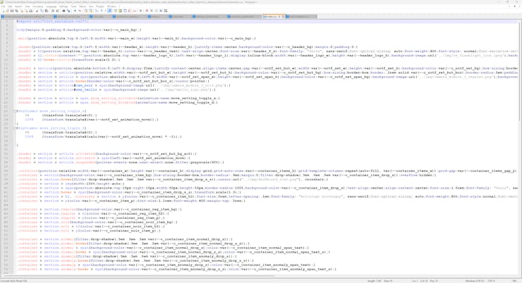
📁 uv_defect_detection_run_inference_w_rasp_5_camera_mod_wide_and_noir.py

⭐ Include the required system and third-party libraries.

⭐ Uncomment to modify the libcamera log level to bypass the libcamera warnings if you want clean shell messages while running inferences.

import serial
import cv2
from picamera2 import Picamera2, Preview
from time import sleep
from threading import Thread
from edge_impulse_linux.image import ImageImpulseRunner
import os
import datetime
import requests
import json

# Uncomment to disable libcamera warnings whuile collecting data.
#os.environ["LIBCAMERA_LOG_LEVELS"] = "4"

#️⃣ To bundle all the functions to write a more concise script, I used a Python class.

⭐ In the __init__ function:

⭐ Define a picamera2 object addressing the CSI port of the Raspberry Pi camera module 3 Wide.

⭐ Define the output format and size (resolution) of the images captured by the regular camera module 3 to obtain an OpenCV-compatible buffer — RGB888. Then, configure the picamera2 object accordingly.

⭐ Initialize the video stream (feed) produced by the regular camera module 3.

⭐ Define a secondary picamera2 object addressing the CSI port of the Raspberry Pi camera module 3 NoIR Wide.

⭐ Define the output format and size (resolution) of the images captured by the camera module 3 NoIR to obtain an OpenCV-compatible buffer — RGB888. Then, configure the picamera2 object accordingly.

⭐ Initialize the video stream (feed) produced by the camera module 3 NoIR.

⭐ Declare the directory path to access the Edge Impulse FOMO-AD (visual anomaly detection) model.

⭐ Then, based on the previous experiments, define the anomaly (confidence) threshold.

⭐ Declare the circular conveyor plastic carrier (station) number parameters to enable the web dashboard to track plastic objects by carriers while transferring the inference results to it.

⭐ Initialize serial communication between the ATmega328P chip and the Raspberry Pi 5 through the built-in UART GPIO pins.

class uv_defect_detection():
    def __init__(self, model_file):
        # Define the Picamera2 object for communicating with the Raspberry Pi camera module 3 Wide.
        self.cam_wide = Picamera2(0)
        # Define the camera module frame output format and size, considering OpenCV frame compatibility.
        capture_config = self.cam_wide.create_preview_configuration(raw={}, main={"format":"RGB888", "size":(640,640)})
        self.cam_wide.configure(capture_config)
        # Initialize the camera module continuous video stream (feed).
        self.cam_wide.start()
        sleep(2)
        
        # Define the Picamera2 object for communicating with the Raspberry Pi camera module 3 NoIR Wide.
        self.cam_noir_wide = Picamera2(1)
        # Define the camera module NoIR frame output format and size, considering OpenCV frame compatibility.
        capture_config_noir = self.cam_wide.create_preview_configuration(raw={}, main={"format":"RGB888", "size":(640,640)})
        self.cam_noir_wide.configure(capture_config_noir)
        # Initialize the camera module NoIR continuous video stream (feed).
        self.cam_noir_wide.start()
        sleep(2)
        
        # Define the required configurations to run the provided Edge Impulse FOMO-AD (visual anomaly detection) model.
        self.dir_path = os.path.dirname(os.path.realpath(__file__))
        self.model_file = os.path.join(self.dir_path, model_file)
        self.anomaly_threshold = 8
        
        # Declare the circular conveyor station number to track plastic objects after running inferences.
        self.station_num = 0
        self.total_station_num = 11
        
        # Initialize serial communication between ATMEGA328P and Raspberry Pi 5 through the built-in UART GPIO pins.
        self.ATMEGA328 = serial.Serial("/dev/ttyAMA0", 9600, timeout=1000)
        sleep(3)
		
		...

⭐ In the display_camera_feeds function:

⭐ Obtain the latest frame generated by the regular camera module 3.

⭐ Show the obtained frame on the screen via the built-in OpenCV tools.

⭐ Then, obtain the latest frame produced by the camera module 3 NoIR and show the retrieved frame in a separate window on the screen via the built-in OpenCV tools.

⭐ Stop both camera feeds (regular Wide and NoIR Wide) and terminate individual OpenCV windows once requested.

def display_camera_feeds(self):
        # Display the real-time video stream (feed) produced by the camera module 3 Wide.
        self.latest_frame_wide = self.cam_wide.capture_array()
        cv2.imshow("UV-based Surface Defect Detection [Wide Preview]", self.latest_frame_wide)
        # Display the real-time video stream (feed) produced by the camera module 3 NoIR Wide.
        self.latest_frame_noir = self.cam_noir_wide.capture_array()
        cv2.imshow("UV-based Surface Defect Detection [NoIR Preview]", self.latest_frame_noir)            
        # Stop all camera feeds once requested.
        if cv2.waitKey(1) & 0xFF == ord('q'):
            cv2.destroyAllWindows()
            self.cam_wide.stop()
            self.cam_wide.close()
            print("\nWide Camera Feed Stopped\n")
            self.cam_noir_wide.stop()
            self.cam_noir_wide.close()
            print("\nWide NoIR Camera Feed Stopped!\n")

⭐ In the camera_feeds function, initiate the loop to show the latest frames produced by the regular Wide and NoIR Wide camera modules consecutively to observe the real-time video streams (feeds) simultaneously.

def camera_feeds(self):
        # Start the camera video streams (feeds) in a loop.
        while True:
            self.display_camera_feeds()

⭐ In the run_inference function:

⭐ Initiate the integrated Edge Impulse ImageImpulseRunner to utilize the provided Edge Impulse FOMO-AD visual anomaly detection model converted to an EIM binary for Linux (AARCH64).

⭐ If requested, print the detailed model information.

⭐ According to the passed camera type, obtain the latest camera frame generated by the camera module 3 Wide or the camera module 3 NoIR Wide for running an inference.

⭐ After obtaining the latest frame, generate the required features from the retrieved frame based on the provided model information.

#️⃣ Since the Edge Impulse FOMO-AD (visual anomaly detection) models categorize given image samples by producing individual cells (grids) according to the dichotomy between the normal image sample features with which the model was trained and the passed features, there can only be two different classes in relation to the declared anomaly threshold: anomaly and no anomaly.

#️⃣ To identify the plastic surface anomalies, I compared the produced mean visual anomaly values with the anomaly threshold score pinpointed by running the model on the testing samples repeatedly via the Edge Impulse Studio.

⭐ First, after running the inference, obtain the individual cells (grids) with their assigned labels and anomaly scores.

⭐ For each cell with the anomaly label, check whether its anomaly score is greater than the given threshold.

⭐ If so, in relation to the provided anomaly range, draw cells on the inference image in three different colors (BGR) to showcase the extent of defective and damaged surface areas.

⭐ After processing the anomaly score information successfully, update the circular conveyor plastic carrier (station) number and save the processed and modified inference image to the inference_results folder.

⭐ Finally, transfer the generated inference information to the circular conveyor web dashboard, which registers the transferred information into the associated MariaDB database table.

def run_inference(self, cam_type, __debug):
        # Run an inference with the provided FOMO-AD model to detect plastic surface defects via visual anomaly detection based on UV-exposure.
        with ImageImpulseRunner(self.model_file) as runner:
            try:
                detected_class = ""
                # If requested, print the information of the Edge Impulse FOMO-AD model converted to a Linux (AARCH64) application (.eim).
                model_info = runner.init()
                if(__debug): print('\nLoaded runner for "' + model_info['project']['owner'] + ' / ' + model_info['project']['name'] + '"')
                labels = model_info['model_parameters']['labels']
                # According to the passed camera type, obtain the latest camera frame generated by the camera module 3 Wide or the camera module 3 NoIR Wide for running an inference.
                latest_frame = self.latest_frame_wide if (cam_type == "regular") else self.latest_frame_noir
                # After obtaining the latest frame, modify the retrieved frame based on the provided model requirements in order to generate accurate features.
                features, cropped = runner.get_features_from_image(latest_frame)
                res = runner.classify(features)
                # Since the Edge Impulse FOMO-AD (visual anomaly detection) models categorize given image samples by individual cells (grids)
                # according to the dichotomy between the pretrained anomaly image samples and the passed image sample, there can only be two different classes: anomaly and no anomaly.
                # To identify the plastic surface anomalies, I compared the produced mean visual anomaly values with the anomaly threshold score pinpointed by running the model on the testing samples repeatedly via the Edge Impulse Studio.
                if res["result"]["visual_anomaly_mean"] >= self.anomaly_threshold:
                    detected_class = "anomaly"
                    # Obtain the cells with their assigned labels and anomaly scores evaluated by the FOMO-AD (visual anomaly detection) model.
                    intensity = ""
                    anomaly_range = 3
                    for cell in res["result"]["visual_anomaly_grid"]:
                        # Draw each cell assigned with an anomaly score greater than the given anomaly threshold on the inference image.
                        if cell["label"] == "anomaly" and cell["value"] >= self.anomaly_threshold:
                            # Utilize different colors (BGR) for the cells to showcase the extent of defective and damaged surface areas.
                            cell_c = (255, 26, 255)
                            if(cell["value"] >= self.anomaly_threshold+anomaly_range and cell["value"] < self.anomaly_threshold+(2*anomaly_range)): cell_c = (26, 163, 255)
                            elif(cell["value"] >= self.anomaly_threshold+(2*anomaly_range)): cell_c = (0, 0, 255)
                            # Draw the cell.
                            cv2.rectangle(cropped, (cell["x"], cell["y"]), (cell["x"]+cell["width"], cell["y"]+cell["height"]), cell_c, 2)
                else:
                    detected_class = "normal"
                # After running the provided FOMO-AD model successfully:
                if detected_class != "":
                    if(__debug): print("\nFOMO-AD Model Detection Result => " + detected_class + "\n")
                    # Update the circular conveyor station number accordingly.
                    self.station_num += 1
                    if(self.station_num > self.total_station_num): self.station_num = 1
                    # Save the produced and modified inference image to the inference_results folder.
                    file_name, date = self.save_inference_result_img(cam_type, detected_class, cropped, __debug)
                    # Register the given inference information to the surface defect detection web dashboard.
                    self.register_inference_info(cam_type, detected_class, file_name, date, __debug)
            # Stop the running inference.    
            finally:
                if(runner):
                    runner.stop()

⭐ In the save_inference_result_img function:

⭐ Define the file name and path of the provided inference image by applying the passed inference parameters.

⭐ Then, save the passed inference image to the inference_results folder.

⭐ Return the produced file name and file creation time for further usage.

def save_inference_result_img(self, cam_type, detected_class, passed_image, __debug):
        # According to the provided image information, save the passed inference image to the inference_results folder.
        date = datetime.datetime.now().strftime("%Y_%m_%d_%H_%M_%S")
        file_name = "inference_results/{}_{}_{}__{}.jpg".format(detected_class, cam_type, self.station_num, date)
        cv2.imwrite(file_name, passed_image)
        if(__debug): print("Inference image successfully saved: " + file_name)
        return file_name, date

⭐ In the register_inference_info function:

⭐ By making an HTTP POST request in the form of a JSON object literal, transfer the passed inference information to the circular conveyor web dashboard.

def register_inference_info(self, cam_type, detected_class, file_name, date, __debug):
        # Register the passed inference information to the surface defect detection web dashboard.
        url = "http://localhost/surface_defect_detection_dashboard/assets/anomaly_update.php"
        data = {"anomaly_log[cam_type]": cam_type, "anomaly_log[detection]": detected_class, "anomaly_log[img_file]": file_name, "anomaly_log[station_num]": self.station_num, "anomaly_log[detection_time]": date}
        r = requests.post(url, data=data)
        if(__debug): print("Inference information successfully registered to the web dashboard! Server response: " + r.text)

⭐ In the consecutive_inferences function, run inferences with the latest frames produced by the regular Wide camera module and the NoIR Wide camera module consecutively.

def consecutive_inferences(self):
        self.run_inference("regular", True)
        sleep(1)
        self.run_inference("noir", True)

⭐ In the obtain_ATMEGA328_data_packets function:

⭐ Obtain the data packets transferred by the ATmega328P chip via serial communication (UART) continuously.

⭐ If the run command is received, run inferences with both camera modules (regular and NoIR) consecutively.

⭐ Then, inform the ATmega328P chip once the inferences are completed by sending the associated data packet (char).

⭐ If the test command is received, send the associated data packet (char) to ensure that the two-way serial data transmission is working as anticipated.

def obtain_ATMEGA328_data_packets(self):
        # Obtain the data packets transferred by ATMEGA328P via serial communication continuously.
        while True:
            sleep(.5)
            if self.ATMEGA328.in_waiting > 0:
                data_packet = self.ATMEGA328.readline().decode("utf-8", "ignore").rstrip()
                print("Received data packet [ATMEGA328P]: " + data_packet)
                if(data_packet.find("run") >= 0):
                    # Run inferences with the camera module 3 Wide (regular) and the camera module 3 NoIR Wide (noir) consecutively.
                    self.consecutive_inferences()
                    # Then, inform ATMEGA328P of the completed inferences.
                    self.ATMEGA328.write("s".encode("utf-8"))
                if(data_packet.find("test") >= 0):
                    # Testing serial connection status.
                    self.ATMEGA328.write("w".encode("utf-8"))
                    print("Serial connection test...\n")

#️⃣ As the program needs to check for data packets transferred by the ATmega328P chip via serial communication (UART) without interruptions, it would not be feasible to check for data packets while running the real-time video streams generated by OpenCV in the same operation (runtime), which processes the latest frames produced by the regular Wide and NoIR Wide camera modules continuously. Therefore, I utilized the built-in Python threading module to run multiple operations concurrently and synchronize them.

⭐ Define the uv_defect_detection class object.

⭐ Declare and initialize a Python thread for running the real-time video streams (feeds) produced by the regular camera module 3 and the camera module 3 NoIR.

⭐ Outside of the video streams operation (thread), check for the latest data packets transferred by the ATmega328P chip via serial communication (UART).

uv_defect_detection_obj = uv_defect_detection("fomo_ad_model/ai-driven-plastic-surface-defect-detection-via-uv-exposure-linux-aarch64-v1.eim")

# Declare and initialize a Python thread for the camera module 3 Wide and the camera module 3 NoIR Wide video streams (feeds).
Thread(target=uv_defect_detection_obj.camera_feeds).start()

# Declare and initialize a Python thread for continuous communication with ATMEGA328P via serial communication.
uv_defect_detection_obj.obtain_ATMEGA328_data_packets()

 

 

 

 

 

 

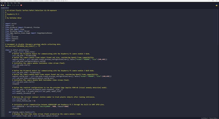
Circular Conveyor - Step 9: Configuring Raspberry Pi Connect and preparing the circular conveyor mechanism for final experiments

Before completing the assembly of the circular conveyor mechanism, I ensured all of the circular conveyor web dashboard functions were working as expected. Even though I explained the conveyor part assembly before the web dashboard development process to write a concise tutorial, concluding the circular conveyor mechanism was not a linear process: I needed to work on component assembly, part redesigns, and dashboard development simultaneously to build the final version of the circular conveyor.

 

 

After completing the final version of the circular conveyor, I could easily connect to the Raspberry Pi 5 without utilizing a screen via the Secure SHell (SSH) protocol to access the Python program running inferences with the FOMO-AD visual anomaly detection model and showcasing the real-time camera feeds produced by the regular camera module 3 Wide and the camera module 3 NoIR Wide. Nonetheless, the SSH connection was not feasible for me to document the features of the final version of the circular conveyor mechanism, since I wanted to screen record the real-time camera feeds for the demonstration videos. In this regard, I decided to employ Raspberry Pi Connect to access my Raspberry Pi desktop and command line directly from any browser. Since Raspberry Pi Connect is officially developed by Raspberry Pi and integrated into the Raspberry Pi OS, it is a highly secure and simple remote access solution.

#️⃣ Even though the rpi-connect package should be installed by default in Raspberry Pi OS (Bookworm or later), I tried to reinstall it to see if there were any dependency issues.

sudo apt install rpi-connect

 

#️⃣ Then, I initiated Raspberry Pi Connect via the terminal (command line).

rpi-connect on

 

#️⃣ After starting Raspberry Pi Connect, I needed to associate my Raspberry Pi 5 with my Connect account. Thus, I started the Connect account sign-in procedure via the terminal.

rpi-connect signin

 

#️⃣ Then, I navigated to the Connect sign-in page on the browser and created a new account.

 

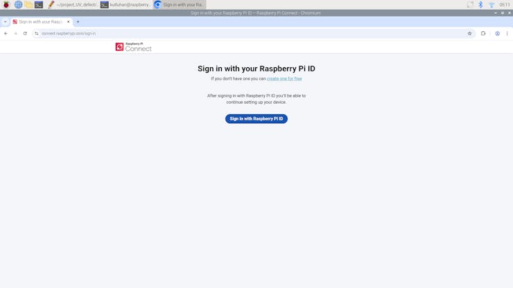
#️⃣ After creating my Connect account successfully, I opened the verification link on the terminal, generated by the rpi-connect package, to verify my device.

 

#️⃣ After naming and verifying my Raspberry Pi 5, it was signed in to the Connect service without any problems.

 

 

After configuring Raspberry Pi Connect, the circular conveyor mechanism was ready for me to conduct final experiments to showcase all its features.

Thanks to the separate UV light source mounts, I was able to switch the UV light sources for both camera modules (regular Wide and NoIR Wide) effortlessly while conducting final experiments.

Nevertheless, I decided to only utilize the color gel filters with the camera module 3 NoIR Wide and the glass UV bandpass filter with the regular camera module 3 Wide. Since the UV bandpass filter blocks the IR (infrared) spectrum as well as the UV spectrum, it renders the no infrared filter hardware characteristic of the NoIR variant ineffectual.

 

 

 

 

 

 

 

 

 

Circular Conveyor Features: Capturing UV-applied plastic surface images with both camera module 3 versions (regular Wide and NoIR Wide) while logging the applied experiment parameters

⛓️ ⚙️ 🔦 🟣 The circular conveyor mechanism lets the user capture UV-applied plastic surface images with both camera modules (regular Wide and NoIR Wide) and record the applied experiment parameters to the file names by simply entering Python inputs in this format:

0, 0, 2, 3, 2, 0

[cam_focal_surface_distance], [uv_source_wavelength], [material], [filter_type], [surface_defect], [camera_type]

cam_focal_surface_distance: the distance between the camera focal point and the center of the target plastic object

• 0: 3cm
• 1: 5cm

uv_source_wavelength: the wavelength of the UV light source applied to the plastic object surface

• 0: 275nm
• 1: 365nm
• 2: 395nm

material: the filament (material) type of the target plastic object

• 0: matte_white
• 1: matte_khaki
• 2: shiny_white
• 3: fluorescent_blue
• 4: fluorescent_green

filter_type: the filter type attached to the selected camera's external filter lens

• 0: gel_low_tr
• 1: gel_medium_tr
• 2: gel_high_tr
• 3: uv_bandpass

surface_defect: the surface defect stage of the target plastic object

• 0: none
• 1: high
• 2: extreme

camera_type: the selected camera to capture a new UV-applied plastic surface image

• 0: wide
• 1: wide_noir

 

 

 

⛓️ ⚙️ 🔦 🟣 Since the circular conveyor mechanism shows the real-time camera feeds produced by the regular camera module 3 Wide and the camera module 3 NoIR Wide, it enables the user to capture precise and high-quality UV-applied images.

⛓️ ⚙️ 🔦 🟣 It also saves the collected images by registering the given experiment parameters to their file names under this directory tree, leading to sorting images effortlessly for further model training or testing.

• wide
• extreme
• high
• none
• wide_noir
• extreme
• high
• none

 

 

 

 

 

 

 

 

⛓️ ⚙️ 🔦 🟣 Even though I had already trained my FOMO-AD visual anomaly detection model with the image samples collected via the data collection rig based on Raspberry Pi 4, it was crucial to experiment with capturing samples with Raspberry Pi 5, utilizing a dual-camera setup, to ensure the FOMO-AD model would produce consistent anomaly results.

 

 

 

 

 

 

 

 

 

Circular Conveyor Features: Adjusting circular conveyor attributes and analyzing the behavior of system components

⛓️ ⚙️ 🔦 🟣 On the interface of the circular conveyor mechanism, the user can change the highlighted interface option by pressing the control button A and the control button C.

⛓️ ⚙️ 🔦 🟣 Once an interface option is highlighted, in other words, having the current cursor position, the user can activate (initiate) the highlighted option by pressing the control button B.

⛓️ ⚙️ 🔦 🟣 After activating an interface option, the user can terminate the ongoing task and return to the home screen by pressing the control button D.

• [A] ➡ Down
• [C] ➡ Up
• [B] ➡ Activate (Select)
• [D] ➡ Exit (Terminate)

 

⛓️ ⚙️ 🔦 🟣 Once the Adjust Interface option is activated, the user can adjust the two potentiometer values mapped according to the associated conveyor configurations.

⛓️ ⚙️ 🔦 🟣 The first potentiometer value (mapped) denotes the speed parameter, managing how fast the stepper motors rotate the sprockets. Once the user presses the control button A, the latest value of the first potentiometer becomes the speed parameter.

⛓️ ⚙️ 🔦 🟣 The second potentiometer value (mapped) denotes the station pending time parameter, which is the intermission to give camera modules time to focus before running the successive inference. Once the user presses the control button C, the latest value of the second potentiometer becomes the station pending time parameter.

 

 

 

 

 

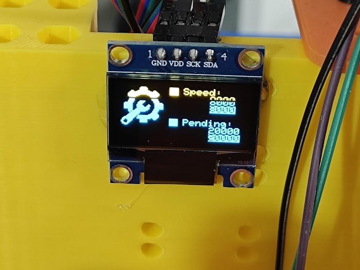
⛓️ ⚙️ 🔦 🟣 Once the Check Interface option is activated, the user can rotate the stepper motors driving sprockets simultaneously to review the circular conveyor movement and the chain tension.

• [A] ➡ One step clockwise
• [C] ➡ One step counterclockwise

⛓️ ⚙️ 🔦 🟣 Furthermore, the user can inspect the real-time raw readings yielded by two magnetic Hall-effect sensor modules to review whether the neodymium magnets attached to the bottom of the plastic object carriers are precisely aligned with the sensor's center point.

 

 

 

 

 

 

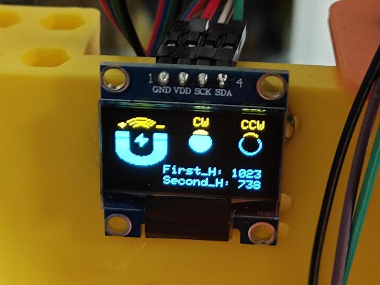
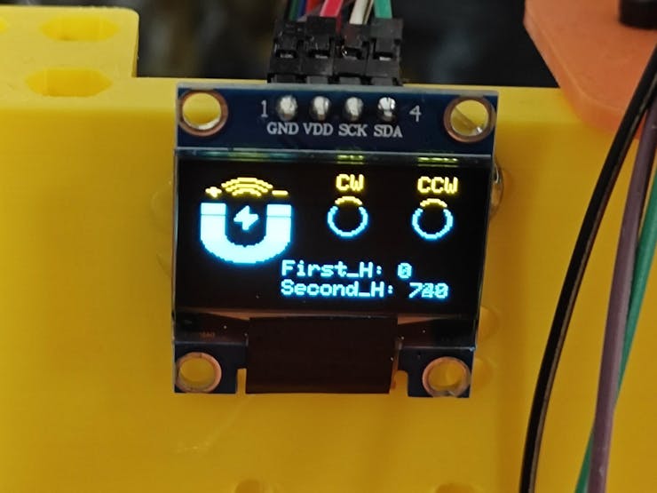
⛓️ ⚙️ 🔦 🟣 Once the Serial Interface option is activated, the conveyor interface shows the response (latest received data packet) as 'o' (ok), meaning the system is ready.

⛓️ ⚙️ 🔦 🟣 Then, the user can transfer specific commands from the conveyor interface (ATmega328P) to the Raspberry Pi 5 via serial communication.

 

 

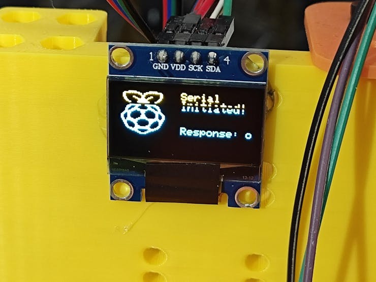
⛓️ ⚙️ 🔦 🟣 Once the user presses the control button A, the interface transfers the test command to the Raspberry Pi 5 and waits for the response to show it on the screen according to the success of two-way data transmission — 'w' (working) or 'n' (none).

 

 

 

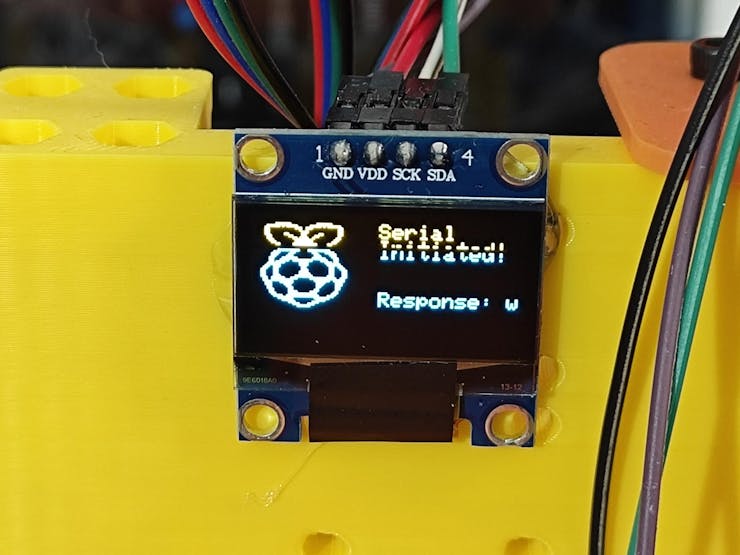
⛓️ ⚙️ 🔦 🟣 Once the user presses the control button C, the interface transfers the run command, leading the Raspberry Pi 5 to run consecutive inferences with the provided FOMO-AD visual anomaly detection model by utilizing images captured by both camera modules (regular Wide and NoIR Wide).

⛓️ ⚙️ 🔦 🟣 Then, the Raspberry Pi 5 modifies the inference images to draw heatmaps and transfers the anomaly detection results to the circular conveyor web dashboard.

⛓️ ⚙️ 🔦 🟣 After running the inferences successfully, the Raspberry Pi 5 informs the conveyor interface (ATmega328P) by sending the associated data packet (char) — 's' (success).

#️⃣ Since the Raspberry Pi 5 and the web dashboard perform the same processes while running inferences manually and automatically, I did not cover them in this step to avoid repetition. Thus, please refer to the following step to review the related Pi 5 and dashboard features.

 

 

 

⛓️ ⚙️ 🔦 🟣 When the user terminates the Serial Interface option, the conveyor interface clears the latest received data packet to restart the manual data transmission procedure.

 

 

 

 

Circular Conveyor Features: Detecting plastic surface anomalies automatically, observing the latest inference results (including heatmaps by grids) via the Twilio-enabled web dashboard, and sorting them by camera type

⛓️ ⚙️ 🔦 🟣 Once the Activate Interface option is activated, the circular conveyor mechanism initiates the automatic plastic surface anomaly detection procedure via UV-exposure.

 

 

⛓️ ⚙️ 🔦 🟣 First, the conveyor interface rotates the stepper motors driving sprockets simultaneously to move the circular conveyor chain continuously but steadily.

⛓️ ⚙️ 🔦 🟣 When both of the magnetic Hall-effect sensor modules detect neodymium magnets attached to the bottom of two successive plastic object carriers simultaneously, the conveyor interface stops the circular conveyor motion immediately, aligning the focal point of the camera modules and the center of the target plastic object surfaces. Then, the interface becomes idle until the given intermission (station pending time) passes, giving both camera modules (regular Wide and NoIR Wide) time to focus on the plastic object surfaces.

 

 

⛓️ ⚙️ 🔦 🟣 After the intermission, the conveyor interface transfers the run command to the Raspberry Pi 5 via serial communication, leading the Raspberry Pi 5 to run consecutive interferences with the provided FOMO-AD visual anomaly detection model by utilizing images produced by the regular camera module 3 Wide and the camera module 3 NoIR Wide.

⛓️ ⚙️ 🔦 🟣 Since the Edge Impulse FOMO-AD (visual anomaly detection) models categorize given image samples by producing individual cells (grids) with assigned labels and anomaly scores, the Raspberry Pi 5 modifies the inference images to draw each cell with an anomaly score higher than the given confidence threshold in three different colors in relation to the provided anomaly range to emphasize the extent of defective and damaged surface areas.

• Pink ➡ Scratched
• Orange ➡ Dented
• Red ➡ Highly damaged

⛓️ ⚙️ 🔦 🟣 After running inferences and modifying the inference images with anomaly scores higher than the given confidence threshold to draw heatmaps, the Raspberry Pi 5 transfers the anomaly detection results to the circular conveyor web dashboard.

 

 

⛓️ ⚙️ 🔦 🟣 While the conveyor chain moves the plastic object carriers automatically, the user can switch UV light sources for both camera modules effortlessly, thanks to the separate UV light source mounts.

• 275 nm
• 365 nm
• 395 nm

 

 

 

 

 

 

 

 

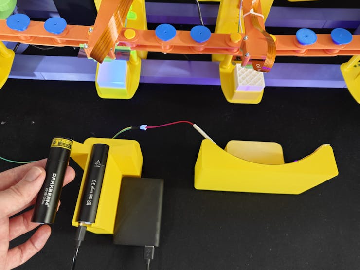
⛓️ ⚙️ 🔦 🟣 Once the user navigates to the conveyor web dashboard, it checks for surface anomaly detection logs (results) from the associated database table. If there are no anomaly detection results yet, the web dashboard informs the user accordingly.

 

 

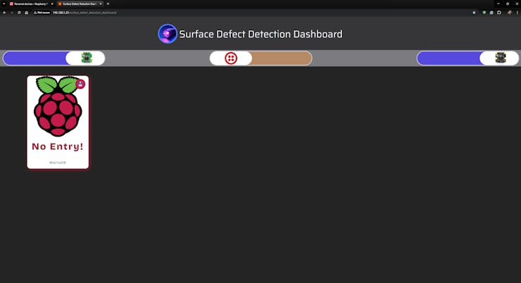
⛓️ ⚙️ 🔦 🟣 Otherwise, the web dashboard generates an HTML card for each surface anomaly result, including the inference date, the inference image, the detected class, and the number of the plastic carrier carrying the target plastic object. Then, the dashboard shows the retrieved anomaly results as HTML cards emphasizing the inference images. Since the web dashboard checks for anomaly results automatically every 2 seconds, the user can review the latest surface anomaly results immediately.

 

 

 

⛓️ ⚙️ 🔦 🟣 The web dashboard allows the user to sort plastic surface anomaly detection results by camera type (regular Wide or NoIR Wide) while obtaining the latest logs from the database table automatically, leading the user to easily track real-time surface anomaly detection results produced by the selected camera module.

⛓️ ⚙️ 🔦 🟣 Once a camera type is disabled, the web dashboard suspends the remaining camera type toggle switch to avoid data omission while sorting surface anomaly detection results.

 

 

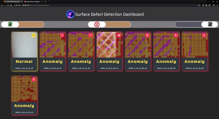
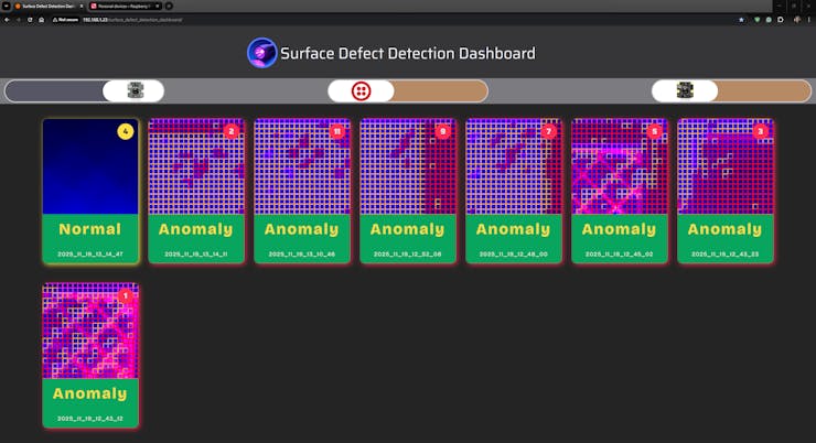
⛓️ ⚙️ 🔦 🟣 As the user enables the Twilio integration, the web dashboard sends an SMS message for each detected plastic surface anomaly via the Twilio SMS API to inform the user.

⛓️ ⚙️ 🔦 🟣 Since the transferred SMS messages include links to the inference images with heatmaps, the user can review the degree of the latest detected plastic surface anomalies effortlessly.

 

 

 

 

 

 

 

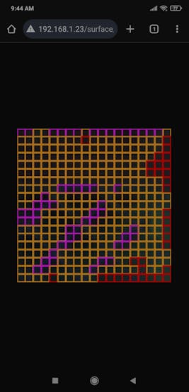
⛓️ ⚙️ 🔦 🟣 Furthermore, the user can review the latest plastic surface anomaly detection results by directly inspecting the inference images since the file names include the exact same information as the HTML cards generated by the web dashboard.

 

📌 normal_noir_5__2025_11_19_13_14_49.jpg

 

 

📌 anomaly_noir_8__2025_11_19_12_25_43.jpg

 

 

 

 

 

 

 

 

 

 

Project GitHub Repository

The project's GitHub repository provides:

 

• The extensive UV-applied plastic surface image dataset
• Code files
• PCB manufacturing files
• Mechanical part and component design files (STL)
• Edge Impulse FOMO-AD visual anomaly detection model (EIM binary for Linux AARCH64)